1. Reference problem#
1.1. Geometry#
According to the modeling \(\mathrm{2D}\) (plane deformation) or \(\mathrm{3D}\), we consider respectively a rectangle or a bar (see Figure 1.1-1).
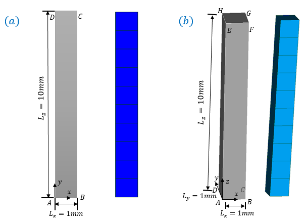
Figure 1.1-a : Geometry and Meshing of a rectangle (a) and a bar (b)
1.2. Material properties#
Elasticity:
\(E=190000\text{MPa}\) |
Young’s module |
\(\mathrm{\nu }=0.3\) |
Poisson’s ratio |
Work hardening curve:
\(R(\mathrm{\kappa })=488.36+57.13(1-\mathrm{exp}(-8613\mathrm{\kappa }))+238.73(1-\mathrm{exp}(-10.39\mathrm{\kappa }))\)
Ductile damage law GTN:
\({q}_{1}=1.5\) |
Model parameter GTN |
\({q}_{2}=1.07\) |
Model parameter GTN |
\({f}_{0}=0.0002i\) |
Initial porosity |
\({f}_{n}=0\) |
Germination Parameter |
\({f}_{c}=0.05\) |
Coalescence porosity |
\(\mathrm{\delta }=3\) |
Coalescence coefficient related to coalescence |
\(c=1N\) |
Non-local parameter |
\(r=5000\mathit{MPa}\) |
Lagrange penalty parameter |
In particular, the distribution of the initial porosity is not homogeneous. It increases with altitude: \({f}_{0}=0.0002i\) where \(i\) refers to the i-th element layer and \(1\le i\le 10\).
In DEFI_MATERIAU, the following information should be filled in:
ELAS |
ECRO_ NL |
GTN |
NON_LOCAL |
|
E = 190000 |
R0= 488.361123569 |
Q1 = 1.5 |
C_ GRAD_VARI = 1 |
|
NU = 0.3 |
R1 = 57.1333673502 |
Q2 = 1.07 |
|
|
GAMMA_1 = 8613 |
|
|||
R2 = 238.731127339 |
|
|||
GAMMA_2 =10.386585592 |
|
1.3. Boundary conditions and loads#
For modeling \(2D\) (plane deformation), the displacements along the \(X\) axis of all the nodes are controlled: \({u}_{x}=5x\), the displacements along the \(Y\) axis of the nodes of the same altitude remain uniform, the node \(A\) is blocked along the \(Y\) axis (see Figure 1.1-1 (a) for geometry).
For modeling \(3D\), the movements along the \(X\) axis of all the nodes are controlled: \({u}_{x}=5x\), the movements along the \(Y\) axis of all the nodes are blocked, the movements along the \(Z\) axis of the nodes of the same altitude remain uniform, the node \(A\) is blocked according to \(Z\). (see Figure 1.1-1 (b) for geometry).
Boundary conditions and loads are imposed this way so that the problem in \(2D\) and the problem in \(3D\) are the same.
The load is imposed using 1000 identical time steps. The pseudo-calculation time is 1.