1. Reference problem#
1.1. Geometry#
According to the modeling \(\mathrm{2D}\) (plane deformation) or \(\mathrm{3D}\), we consider respectively a square or a cube with a side of 0.05 \(\text{mm}\) (see Figure. 1.1-1). Because of the symmetry, only a quarter of the geometry is shown.
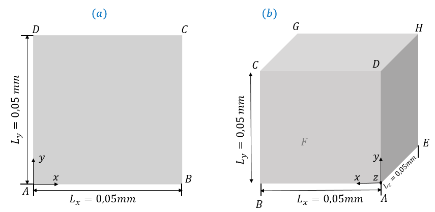
Figure 1.1-a : Geometries of a square**(a) and a cube (b)**
1.2. Material properties#
Elasticity:
\(E=190000\text{MPa}\) |
Young’s module |
\(\mathrm{\nu }=0.3\) |
Poisson’s ratio |
Work hardening curve:
\(R(\mathrm{\kappa })=488.36+57.13(1-\mathrm{exp}(-8613\mathrm{\kappa }))+238.73(1-\mathrm{exp}(-10.39\mathrm{\kappa }))\)
Ductile damage law GTN:
\({q}_{1}=1.5\) |
Model parameter GTN |
\({q}_{2}=1.07\) |
Model parameter GTN |
\({f}_{0}=0.01\) |
Initial porosity |
\({f}_{n}=0\) |
Germination parameter |
\({f}_{c}=0.05\) |
Coalescence porosity |
\(\mathrm{\delta }=3\) |
Coalescence coefficient related to coalescence |
\(c=2.22N\) |
Non-local parameter |
\(r=5000\mathit{MPa}\) |
Lagrange penalty parameter |
In particular, the non-local parameter \(c\) and the penalty parameter \(r\) are only used in the \(\mathit{GTN}\) gradient law.
In DEFI_MATERIAU, the following information should be filled in:
ELAS |
ECRO_ NL |
GTN |
NON_LOCAL |
|
E = 190000 |
R0= 488.361123569 |
Q1 = 1.5 |
C_ GRAD_VARI = 2.22 |
|
NU = 0.3 |
R1 = 57.1333673502 |
Q2 = 1.07 |
|
|
GAMMA_1 = 8613 |
|
|||
R2 = 238.731127339 |
|
|||
GAMMA_2 =10.386585592 |
|
1.3. Boundary conditions and loads#
For modeling \(2D\) (plane deformation), the vertical displacements of all the nodes are controlled: \({u}_{y}=2.2y\), the horizontal displacements are blocked for the side \(\mathit{AD}\) due to symmetry, the horizontal displacements are uniform for the side \(\mathit{BC}\) (see Figure 1.1-1 (a) for the geometry).
For modeling \(3D\), the movements along the \(Y\) axis of all the nodes are controlled: \({u}_{y}=2.2y\), the movements along the \(X\) axis are blocked for the face \(\mathit{ADHE}\) because of the symmetry, the horizontal displacements are uniform for the face \(\mathit{BCGF}\). In addition, the movements along the \(Z\) axis of all nodes are blocked (see Figure 1.1-1 (b) for geometry).
Boundary conditions and loads are imposed in this way so that the problem in \(2D\) and the problem in \(3D\) are the same and homogeneous.
The load is imposed using 1000 identical time steps. The pseudo-calculation time is 1.