1. Reference problem#
1.1. Geometry#
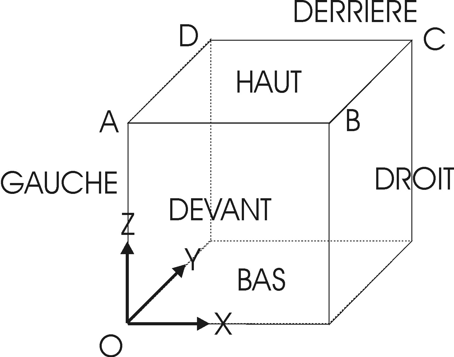
The triaxial test is carried out on a single isoparametric finite element of cubic shape \(\mathit{CUB}8\). The length of each edge is \(1\). The different facets of this cube are mesh groups named \(\mathit{HAUT}\), \(\mathit{BAS}\),, \(\mathit{DEVANT}\), \(\mathit{DERRIERE}\), \(\mathit{DROIT}\), and \(\mathit{GAUCHE}\). The mesh group SYM also contains the mesh groups \(\mathit{BAS}\), \(\mathit{DEVANT}\) and \(\mathit{GAUCHE}\); the group of elements \(\mathit{COTE}\) the mesh groups \(\mathit{DERRIERE}\) and \(\mathit{DROIT}\).
1.2. Material properties#
The elastic properties are:
isotropic compressibility module: \(K=\mathrm{516,2}\mathit{MPa}\)
shear modulus: \(\mathrm{\mu }=\mathrm{238,2}\mathit{MPa}\)
The parameters common to laws MOHR_COULOMB and MohrCoulombas are:
friction angle (FrictionAngle): \(\mathrm{\phi }=33°\)
dilatance angle (dilatancyAngle): \(\mathrm{\psi }=27°\)
cohesion: \({c}_{0}=1\mathit{kPa}\)
The parameters specific to the Mohr-Coulombas law are:
TransitionAngle: \({\mathrm{\theta }}_{T}=29.9°\)
parameter for regulating the criterion in tension (TensionCutoff): \(a=0.25C/\mathrm{tan}(\mathrm{\varphi })\)
hardening hardening parameter (HardeningCoef): \({h}_{C}=0\)
Parameter \({\mathrm{\theta }}_{T}=29.9°\) was chosen so as to approximate the original (singular) Mohr-Coulomb criterion (\({\mathrm{\theta }}_{T}=30°\)); and to ensure that the convergence was not too degraded.
1.3. Boundary conditions and loads#
A triaxial test consists in imposing on the specimen a variation in vertical load while maintaining the lateral pressure constant. It can be drained (the interstitial fluid pressure does not vary during the test) or non-drained (the tap is closed: the fluid interstitial pressure changes in the sample). We are interested here in the drained case, which is simpler, because it does not involve the influence of the interstitial pressure of the fluid and can therefore be modelled by a pure mechanical calculation.
In the model under consideration (case of B and D models), the cubic element represents one eighth of the sample. The boundary conditions are therefore as follows:
Symmetry conditions:
\({u}_{z}=0\) on mesh group \(\mathit{BAS}\)
\({u}_{x}=0\) on mesh group \(\mathit{GAUCHE}\)
\({u}_{y}=0\) on mesh group \(\mathit{DEVANT}\)
Lateral pressure conditions:
\({P}_{n}=1\) on mesh group \(\mathit{COTE}\)
Loading conditions:
\({P}_{n}=1\) on mesh group \(\mathit{HAUT}\) (phase 1)
\({u}_{z}=-1\) on mesh group \(\mathit{HAUT}\) (phase 2)
Charging is carried out in two phases:
**Initialization*. Isotropic loading between \(t\in \left[-2;0\right]s\): the \(p\) pressure on the cell groups \(\mathit{COTE}\) and \(\mathit{HAUT}\) varies from \(0\) to \(p={P}_{0}=50\mathit{kPa}\), the isotropic preconsolidation pressure in the initial state;
triaxial test itself: displacement imposed on the group of elements \(\mathrm{HAUT}\) with \(t\) varying between \(t\in \left[0-30\right]s\) and \({u}_{z}\) varying between \({u}_{z}\in \left[0;-\mathrm{0,3}\right]\mathit{mm}\). The total vertical deformation \({\epsilon }_{\mathit{zz}}\) is \(\mathrm{0,03}\text{\%}\);
1.4. Analytical solution#
The applied loads applied to the cubic sample are represented below:
|
\({\epsilon }_{1}\)
|

Table 1.4-1
It is associated with the potential for plastic flow:
\(g\left({\sigma }_{1},{\sigma }_{3}\right)=\mid {\sigma }_{1}-{\sigma }_{3}\mid +\left({\sigma }_{1}+{\sigma }_{3}\right)\mathrm{sin}\psi -{\mathrm{2c}}_{0}\mathrm{cos}\psi\) (1.4-2)
so that, noting \(t\mathrm{=}\mathrm{sin}\psi\) and \(\xi =\mathit{signe}\left({\sigma }_{1}-{\sigma }_{3}\right)\), the flow law is written as:
\(\mathrm{\{}\begin{array}{c}f({\sigma }_{1},{\sigma }_{3})\mathrm{\ge }0\\ \frac{\mathrm{\partial }g}{\mathrm{\partial }{\sigma }_{1}}\mathrm{=}\dot{{\varepsilon }_{1}^{p}}\mathrm{=}\dot{\lambda }(t+\xi )\\ \frac{\mathrm{\partial }g}{\mathrm{\partial }{\sigma }_{2}}\mathrm{=}\dot{{\varepsilon }_{2}^{p}}\mathrm{=}\dot{{\varepsilon }_{3}^{p}}\mathrm{=}\dot{\lambda }(t\mathrm{-}\xi )\end{array}\) (1.4-3)
where \(\dot{\lambda }\) represents the plastic multiplier. So the two unknowns of the problem are: \({\sigma }_{1}\) (or \({\varepsilon }_{3}\)) and \(\dot{\lambda }\).
1.4.1. Elastic resolution#
The equation is satisfied. We then have:
\(\mathrm{\{}\begin{array}{c}{\sigma }_{1}\mathrm{=}\stackrel{E}{\stackrel{}{(K+\frac{4}{3}G)}}{\varepsilon }_{1}^{e}+2(K\mathrm{-}\frac{2}{3}G){\varepsilon }_{3}^{e}\\ \begin{array}{cc}{\sigma }_{3}\text{=}& (K\mathrm{-}\frac{2}{3}G){\varepsilon }_{1}^{e}+(K\mathrm{-}\frac{2}{3}G){\varepsilon }_{3}^{e}+(K+\frac{4}{3}G){\varepsilon }_{3}^{e}\\ \text{=}& \underset{C}{\underset{\underbrace{}}{(K\mathrm{-}\frac{2}{3}G)}}{\varepsilon }_{1}^{e}+\underset{D}{\underset{\underbrace{}}{2(K+\frac{G}{3})}}{\varepsilon }_{3}^{e}\end{array}\end{array}\) (1.4.1-1)
Knowing that \({\sigma }_{3}\mathrm{=}{\sigma }_{0}\), we can directly deduce from that:
\(\dot{{\varepsilon }_{3}^{e}}\mathrm{=}\mathrm{-}\frac{C}{D}\dot{{\varepsilon }_{1}^{e}}\) (1.4.1-2)
1.4.2. Resolution in a plastic regime#
The equation is satisfied. Let \({\sigma }^{p}\mathrm{=}{\sigma }^{e}\) be the elastic prediction given by the equations, the final constraint \({\sigma }^{\text{+}}\) is written as:
\({\sigma }^{\text{+}}\mathrm{=}\mathrm{ℂ}\mathrm{.}{\varepsilon }^{\text{+}}\mathrm{=}{\sigma }^{p}\mathrm{-}\dot{\lambda }\mathrm{ℂ}\mathrm{.}\overrightarrow{{n}_{g}}\) (1.4.2-1)
where \(\mathrm{ℂ}\mathrm{=}\left[\begin{array}{cc}E& \mathrm{2C}\\ C& D\end{array}\right]\) represents the linear elasticity tensor and \(\overrightarrow{{n}_{g}}\mathrm{=}(t+\xi ,t\mathrm{-}\xi )\).
We calculate the plastic multiplier by writing \(f({\sigma }^{\text{+}})\mathrm{=}0\), that is:
\(\begin{array}{cc}(s+\xi )(K+\frac{4}{3}G){\varepsilon }_{1}^{\text{+}}+2(s+\xi )(K\mathrm{-}\frac{2}{3}G){\varepsilon }_{3}^{\text{+}}& \text{+}\\ (s\mathrm{-}\xi )(K\mathrm{-}\frac{2}{3}G){\varepsilon }_{1}^{\text{+}}+2(s\mathrm{-}\xi )(K+\frac{G}{3}){\varepsilon }_{3}^{\text{+}}& \text{=}2{c}_{0}\mathrm{cos}\phi \end{array}\)
\(\mathrm{\iff }\underset{A}{\underset{\underbrace{}}{2(Ks+G(\xi +\frac{s}{3}))}}{\varepsilon }_{1}^{\text{+}}+\underset{B}{\underset{\underbrace{}}{2(2Ks\mathrm{-}G(\xi +\frac{s}{3}))}}{\varepsilon }_{3}^{\text{+}}\mathrm{=}2{c}_{0}\mathrm{cos}\phi\) (1.4.2-2)
This gives, by replacing:
\(\mathrm{\{}\begin{array}{c}{\varepsilon }_{1}^{\text{+}}\mathrm{=}{\varepsilon }_{1}^{e}\mathrm{-}\dot{\lambda }(t+\xi )\\ {\varepsilon }_{3}^{\text{+}}\mathrm{=}{\varepsilon }_{3}^{e}\mathrm{-}\dot{\lambda }(t\mathrm{-}\xi )\end{array}\) (1.4.2-3)
In, we get: \(\dot{\lambda }\underset{\mathit{BB}}{\underset{\underbrace{}}{\left[A(t+\xi )+B(t\mathrm{-}\xi )\right]}}\mathrm{=}\mathrm{-}2{c}_{0}\mathrm{cos}\phi +A{\varepsilon }_{1}^{e}+B{\varepsilon }_{3}^{e}\mathrm{=}f({\sigma }^{e})\),
That is: \(\dot{\lambda }\mathrm{=}\frac{f({\sigma }^{e})}{\mathit{BB}}\) (1.4.2-4)
1.4.3. Correcting the imbalance#
We need to check \({\sigma }_{3}^{\text{+}}={\sigma }_{0}\). We assume a small virtual variation \(\delta\) of the solution. We are looking for the expression for \(\delta {\sigma }_{3}^{\text{+}}\), that is:
\(\delta {\sigma }_{3}^{\text{+}}=C\delta {\epsilon }_{1}^{e}+E\delta {\epsilon }_{3}^{e}-\delta \dot{\lambda }C\left(t+\xi \right)-\delta \dot{\lambda }E\left(t-\xi \right)\) (1.4.3-1)
Knowing that \(\dot{\lambda }\) is given by, we have: \(\delta \dot{\lambda }=\frac{A}{\mathit{BB}}\delta {\epsilon }_{1}^{e}+\frac{B}{\mathit{BB}}\delta {\epsilon }_{3}^{e}\) (1.4.3-2)
that we report in. This then gives:
\(\delta {\sigma }_{3}^{\text{+}}=\left[C-A\frac{C\left(t+\xi \right)+E\left(t-\xi \right)}{\mathit{BB}}\right]\delta {\epsilon }_{1}^{e}+\left[D-B\frac{C\left(t+\xi \right)+E\left(t-\xi \right)}{\mathit{BB}}\right]\delta {\epsilon }_{3}^{e}\) (1.4.3-3)
During the Newton process, we are looking for a new value of \(\delta {\epsilon }_{3}\) knowing that \(\delta {\epsilon }_{1}=0\) (it is the imposed load, which cannot be false). This value is such that the imbalance \({\sigma }_{0}-{\sigma }_{3}^{\text{+}}\) is corrected, either: \(\frac{\partial {\sigma }_{3}^{\text{+}}}{\partial {\epsilon }_{3}}\delta {\epsilon }_{3}={\sigma }_{0}-{\sigma }_{3}^{\text{+}}\), or, using: \(\delta {\epsilon }_{3}=\frac{{\sigma }_{0}-{\sigma }_{3}^{\text{+}}}{D-B\frac{C\left(t+\xi \right)+E\left(t-\xi \right)}{\mathit{BB}}}\) (1.4.3-4)
1.4.4. Newton’s resolution process#
The resolution process is written as follows:
At the \(t\) time step such as \({\varepsilon }_{1}\mathrm{=}F(t)\): |
||
1 Calculate \({\sigma }_{1}^{p}\) and \({\sigma }_{3}^{p}\) using and |
||
2 As long as \(\mathrm{\mid }{\sigma }_{0}\mathrm{-}{\sigma }_{3}^{\text{+}}\mathrm{\mid }>\epsilon\), perform: |
||
3 |
If \(f({\sigma }_{1}^{p},{\sigma }_{3}^{p})<0\), then OK. \({\sigma }_{1}^{\text{+}}\mathrm{=}{\sigma }_{1}^{p}\) and \({\sigma }_{3}^{\text{+}}\mathrm{=}{\sigma }_{3}^{p}\) and go to 5 |
|
4 |
If \(f({\sigma }_{1}^{p},{\sigma }_{3}^{p})\mathrm{\ge }0\), then NOOK: Calculate \(\dot{\lambda }\) using Calculate \({\varepsilon }_{1}^{\text{+}}\) and \({\varepsilon }_{3}^{\text{+}}\) using Calculate \({\sigma }_{1}^{\text{+}}\) and \({\sigma }_{3}^{\text{+}}\) using |
|
5 |
Calculate \(\delta {\varepsilon }_{3}\) using Update \({\varepsilon }_{3}^{\text{+}}\), \({\sigma }_{1}^{\text{+}}\), and \({\sigma }_{3}^{\text{+}}\) and go to 2 |
|
Table 1.4.4-1 : Resolution procedure for the triaxial test with the Mohr-Coulomb law.
The calculation of the analytical solution is called by the function Triaxial_ DRcontenue in the bibpyt/Contrib/essai_triaxial.py file.
1.4.5. Coherent tangent matrix#
For verification purposes, it is possible to show the coherent tangent matrix of the problem.
In addition to the equation, we also get the following expression for \(\delta {\sigma }_{1}^{\text{+}}\):
\(\delta {\sigma }_{1}^{\text{+}}=\left[E-A\frac{E\left(t+\xi \right)+C\left(t-\xi \right)}{\mathit{BB}}\right]\delta {\epsilon }_{1}^{e}+\left[C-B\frac{E\left(t+\xi \right)+C\left(t-\xi \right)}{\mathit{BB}}\right]\delta {\epsilon }_{3}^{e}\) (1.4.5-1)
So the expression for the coherent tangent matrix \(\mathit{DSDE}\) is written as:
\(\mathit{DSDE}\mathrm{=}\left[\begin{array}{cc}E\mathrm{-}A\frac{E(t+\xi )+C(t\mathrm{-}\xi )}{\mathit{BB}}& C\mathrm{-}B\frac{E(t+\xi )+C(t\mathrm{-}\xi )}{\mathit{BB}}\\ C\mathrm{-}A\frac{C(t+\xi )+E(t\mathrm{-}\xi )}{\mathit{BB}}& E\mathrm{-}B\frac{C(t+\xi )+E(t\mathrm{-}\xi )}{\mathit{BB}}\end{array}\right]\) (1.4.5-2)
1.5. Results#
The solutions are post-treated at point \(C\) for the terms of vertical \({\sigma }_{\mathit{zz}}\) and horizontal stress \({\sigma }_{\mathit{xx}}\), as well as those of plastic volume deformation \({\epsilon }_{v}^{p}\) and plastic deviatoric deformation \(\mid {\epsilon }_{d}^{p}\mid =\sqrt{\frac{3}{2}\left(\epsilon -\frac{{\epsilon }_{v}^{p}}{3}I\right)\mathrm{:}\left(\epsilon -\frac{{\epsilon }_{v}^{p}}{3}I\right)}\).