1. Reference problem#
1.1. Geometry#
For modeling A, the shear test is carried out on a single isoparametric finite element of square shape QUAD8, a cell group called \(\mathrm{BLOC}\). The length of each edge is \(\mathrm{1m}\). The different sides of this square are mesh groups named \(\mathrm{HAUT}\), \(\mathrm{BAS}\), \(\mathrm{DROIT}\), and \(\mathrm{GAUCHE}\). The group of elements \(\mathrm{COTE}\) also contains the mesh groups \(\mathrm{DROIT}\) and \(\mathrm{GAUCHE}\); the mesh group \(\mathrm{APPUI}\) the mesh group \(\mathrm{BAS}\).
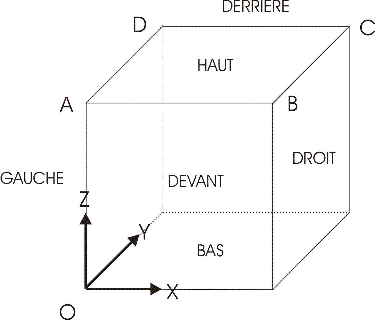
For modeling B the test is carried out on a single isoparametric finite element of cubic shape HEXA8. The length of each edge is 1. The different facets of this cube are mesh groups named \(\mathrm{HAUT}\), \(\mathrm{BAS}\),, \(\mathrm{DEVANT}\), \(\mathrm{ARRIERE}\), \(\mathrm{DROIT}\), and \(\mathrm{GAUCHE}\).
1.2. Material properties of Hostun sand#
The elastic properties are:
isotropic compressibility module: \(K=148\mathit{MPa}\)
shear modulus: \(\mathrm{\mu }=68\mathit{MPa}\)
The equivalent orthotropic elastic properties are:
\({E}_{L}={E}_{T}={E}_{N}=176.906250\mathit{MPa}\)
\({G}_{L}={G}_{T}={G}_{N}=68\mathit{MPa}\)
\({\mathrm{\nu }}_{L}={\mathrm{\nu }}_{T}={\mathrm{\nu }}_{N}=0.30078125\)
The anelastic properties (Hujeux model) come from K.Hamadi’s thesis thesis [:ref:` **2 <**2>`] ** and correspond to low-density Hostun sand:
power of the nonlinear elastic law: \({n}_{e}=0.\) (linear elastic)
\(\beta =30.\)
\(d=2.5\)
\(b=0.2\)
friction angle: \(\phi =33°\)
characteristic angle: \(\Psi =33°\)
critical pressure: \({P}_{\mathit{CO}}=-400\mathit{kPa}\)
reference pressure: \({P}_{\mathrm{ref}}=-1000\mathrm{kPa}\)
elastic radius of the isotropic mechanism: \({r}_{\mathrm{ela}}^{s}={10}^{-4}\)
elastic radius of the deviatory mechanism: \({r}_{\mathrm{ela}}^{d}=0.01\)
\({a}_{\mathrm{mon}}=0.017\)
\({a}_{\mathrm{cyc}}=0.0001\)
\({c}_{\mathrm{mon}}=0.08\)
\({c}_{\mathrm{cyc}}=0.04\)
\({r}_{\mathrm{hys}}=0.05\)
\({r}_{\mathrm{mob}}=0.9\)
\({x}_{m}=1.\)
\(\mathrm{dila}=1.\)
1.3. Boundary conditions and loads#
The shear test presented here is carried out using D_ PLAN modeling (A modeling) and 3D modeling (B modeling).
For modeling A, the movements normal to the study plan are zero. A vertical displacement is imposed on the specimen while maintaining the lateral pressure constant in the study design. In the model under consideration, the square element represents a quarter of the sample. The boundary conditions are therefore as follows:
Symmetry conditions:
\({u}_{y}=0.\) on mesh group \(\mathrm{BAS}\)
\({u}_{x}=0.\) on mesh group \(\mathrm{GAUCHE}\)
Lateral pressure conditions:
\({P}_{n}=100\mathit{kPa}\) on mesh group \(\mathrm{COTE}\)
Loading conditions:
\({P}_{n}=100\mathit{kPa}\) on mesh group \(\mathrm{HAUT}\)
\({u}_{x}=-1\mathit{mm}\) on mesh group \(\mathrm{HAUT}\)
Charging is carried out in two phases:
An isotropic stress state, \({P}_{o}=100\mathrm{kPa}\), is initially assigned to mesh \(\mathrm{BLOC}\);
A horizontal displacement is imposed on the group of elements \(\mathrm{HAUT}\) and varies between \(t=0.\) and \(t=10.\) from \({u}_{y}=0.\) and \({u}_{x}=-1\mathit{mm}\).
For modeling B, an embedment is imposed on the specimen on the face \(\mathrm{BAS}\) and a horizontal movement along X on the face \(\mathrm{HAUT}\), while maintaining the constant lateral pressure in the lateral faces. The boundary conditions are therefore as follows:
The embedding condition:
\({u}_{x}={u}_{y}={u}_{z}=0\) on mesh group \(\mathit{BAS}\)
Lateral pressure conditions:
\({P}_{n}=100\mathit{kPa}\) on mesh groups \(\mathrm{DEVANT}\), \(\mathrm{ARRIERE}\),, \(\mathrm{DROIT}\), and \(\mathrm{GAUCHE}\).
Loading conditions:
\({P}_{n}=100\mathit{kPa}\) on the \(\mathrm{HAUT}\) mesh group applied from the first moment of calculation and maintained thereafter
\({u}_{x}=-\mathrm{0,2}m\) on the \(\mathrm{HAUT}\) mesh group applied progressively by a ramp function
Charging is therefore carried out in two phases:
An isotropic stress state, \({P}_{o}=100\mathrm{kPa}\), is initially assigned to cells \(\mathrm{HAUT}\), \(\mathrm{DEVANT}\), \(\mathrm{ARRIERE}\), \(\mathrm{DROIT}\) and \(\mathrm{GAUCHE}\). ;
A horizontal displacement according to X is imposed on the group of elements \(\mathrm{HAUT}\) and varies between \(t=0.\) and \(t=10.\) from \({u}_{x}=0.\) and \({u}_{x}=-0.2m\).
1.4. Results#
The solutions are post-treated at point \(C\), in terms of stress \({\mathrm{\sigma }}_{\mathit{xy}}\), total volume deformation \({\varepsilon }_{v}\) and isotropic work-hardening coefficients \(\left({r}_{\text{ela}}^{\text{iso},m}+{r}_{\text{iso}}^{m}\right)\) and deviation \(\left({r}_{\text{ela}}^{d,m}+{r}_{\text{dev}}^{m}\right)\).
1.5. Bibliographical references#
[1] Foucault A. « Modeling the cyclical behavior of earthen structures integrating regulation techniques « . Doctoral thesis, École Centrale Paris, École Centrale Paris, Châtenay Malabry, France, 2010.
[2] Hamadi K. « Modeling bifurcations and instabilities in geomaterials ». PhD thesis, École Centrale Paris, Châtenay Malabry, France, 2006