3. Modeling A: FEM 3D#
3.1. Workflow of the TP#
3.1.1. Meshing#
Healthy mesh
It should be noted that taking into account the symmetries of the problem, only half of the structure is modelled. The healthy structure mesh is provided in the format MED: forma08a_sain.mmed. It is a mesh comprising linear tetrahedra.
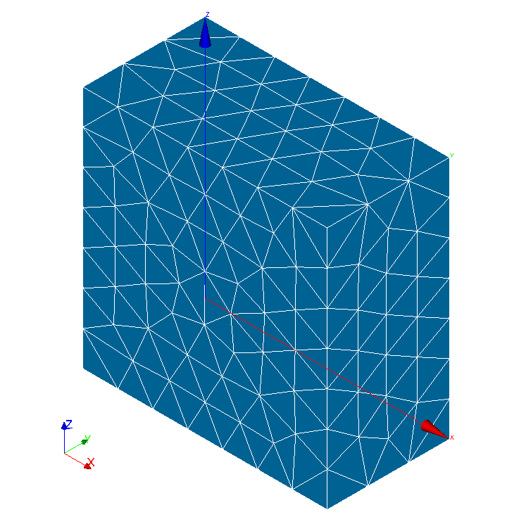
Figure 3.1.1-1: Healthy mesh
Note: This mesh can be built very simply with Salome_Meca by first using the Salome-Meca Geometry module using the New Entity/Primitives/ Box functionality with Dx = 2, Dy = 1 and Dz = 2 then Operations/Transformation/Translation with Dx = -1, Dy = 0 and Dz = -1. Care will be taken to define the geometric groups using the Create Group functionality. Then, with the Mesh module, we generate the mesh using the MG-Tetra and MG- CADSurf algorithms with the default parameters. Remember to import mesh and node groups based on geometric groups.
Cracked mesh
Start Salome_Meca, then choose the Mesh module. In Mesh/SMESH plugins, choose Run Zcracks. the IHM of Zcracks opens.
Zcracks IHM Mesh parameters section:
In the input mesh box, select the file relating to the healthy mesh.
In the Output mesh box, enter a new file name.
In the Minimum size box, enter 0.01. This value corresponds to the target size of the cells close to the crack front, it corresponds to \(h=a/20\). This size is slightly larger than the generally recommended mesh size but allows an initial calculation to be carried out quickly. It will be refined later.
In the Extraction length box, enter 0.5. This value corresponds to 2.5 times the radius of the crack.
Check the LinetoQuad box (the cracked mesh generated will then be a quadratic mesh).
IHM Zcracks Group Section:
Load the group of elements by clicking on the corresponding Load button
Load the surface mesh groups by clicking on the corresponding Load button
Crack section of IHM Zcracks:
Enter the coordinates of the center of the crack: Center: 0 0 0
Enter the components of the normal vector at the crack surface: Normal: 0 0 1
Enter the value of the radius of the crack: Radius: 0.2
Then click the Save button to save the Zcracks data to a file.
Finally, click on the Apply button to start running Zcracks.
The defect is inserted in about 10 s.
Import the cracked mesh into the Mesh module and visualize it. It should look similar to the views below.
Creating and editing groups
Create node groups « D1 » and « D2 » to block rigid body modes.
On the cracked mesh, do « create a group », and create the two nodes « D1 » and « D2 » in manual editing, see.
Rename face groups « SIDE0 » to « LEVREINF » and « SIDE1 » to « LEVRESUP »
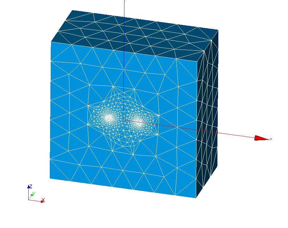
Figure 3.1.1-2: Cracked mesh
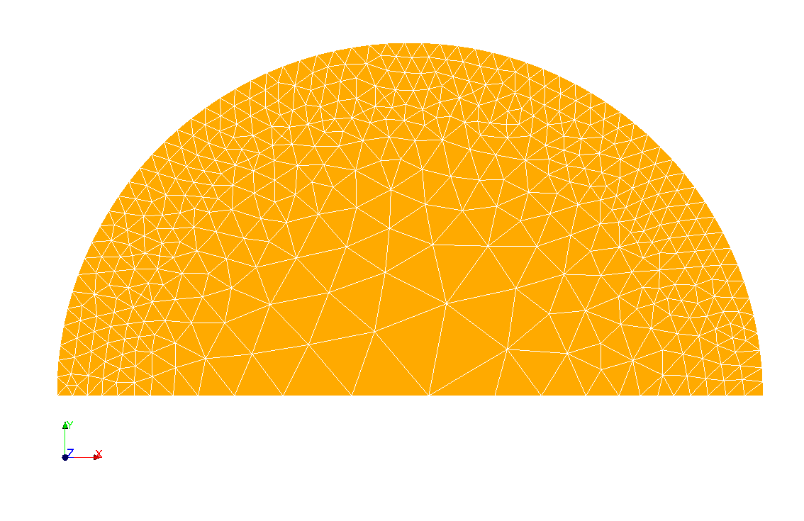
Figure 3.1.1-3: Cracked mesh: zoom on the lips of the crack
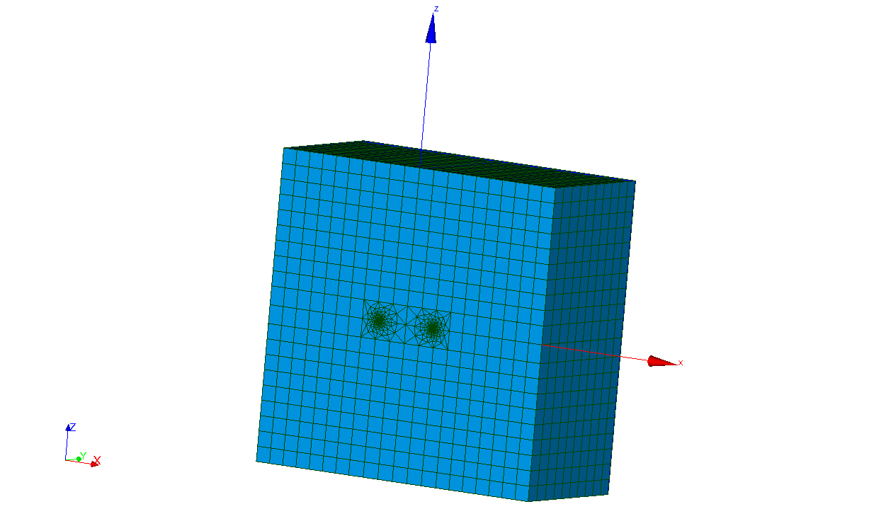
Figure 3.1.1-4: Radiant mesh
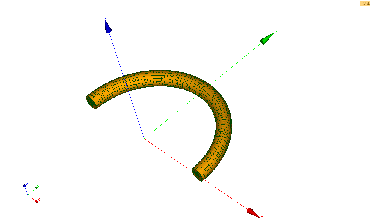
Figure 3.1.1-5: Radiant mesh torus
3.1.2. Creating the batch file without post-processing the break#
Start Salome_Meca, then choose the AsterStudy module. Add the following steps to your case: |
Read a mesh (LIRE_MAILLAGE). Select the cracked mesh obtained earlier and the format MED |
Creating a node group (DEFI_GROUPE). Creating the nodes at the bottom of the crack → Select CREA_GROUP_NO, option = “NOEUD_ORDO”, option = “”, NOM = NO_FOND, GROUP_MA =” FRONT0 “, GROUP_NO_ORIG =” FRONT0B”, GROUP_NO_EXTR =” FRONT0E “. |
Modify the mesh (MODI_MAILLAGE) by transforming the elements at the crack point into Barsoum elements → Select MODI_MAILLE/NOEUD_QUART, GROUP_NO_FOND =” NO_FOND “. |
Modify a mesh (MODI_MAILLAGE). Choose the mesh read earlier and select reuse. Select the ORIE_PEAUpour action to reorient the normals to the faces outside of the mesh (element groups HAUT, BAS, SYME, DROITE, and GAUCHE). |
Assign finite element (AFFE_MODELE). Choose the mechanical phenomenon and the modeling of 3D continuous media (3D) |
Material definition and assignment: Define a material ( DEFI_MATERIAU **) **) and Assign a material ( AFFE_MATERIAU **** )) ** |
Definition of limit conditions and loads: Assign mechanical load **** ( AFFE_CHAR_MECA ): * Symmetry on the symmetry plane “SYME” (Enforce DOF); * Blocking rigid modes (Enforce DOFsur the GROUP_NO “D1” and “D2”); * Applying traction on “HAUT”, “BAS”, “”, “DROITE”, and “GAUCHE” (FORCE_FACE) |
Elastic problem solving: Static mechanical analysis **** (**** MECA_STATIQUE **); |
For visualization with Paravis: * Calculation of the extrapolated constraint field to the nodes (CALC_CHAMP, option “CONTRAINTE” with the field “SIGM_NOEU”) * Calculation of the equivalent stress field (CALC_CHAMP, option “CRITERES” with the field “SIEQ_NOEU”) To do this, we will enrich the concept resulting from MECA_STATIQUE by using the same concept name. |
Printing results in format MED: Results output (IMPR_RESU). |
Visualize the displacement fields and constraints obtained in Paravis |
3.1.3. Post-treatment for breakup#
In order to separate calculation and post-processing, you can add a new stage to your case study. |
Define the crack bottom **** (**** DEFI_FOND_FISS **** ) . Define the crack background in DEFI_FOND_FISSà from the bottom mesh group FRONT0 and the lips LEVREINFet LEVRESUP. |
Calculating K **** and G**** with CALC_G (OPTION =”G, K”). Complete the information on field THETA: * the description of the crack using the keyword FISSURE * the radii of the crown of the theta field (R_INF, R_SUP) (,), to be defined according to the mesh used. By default, R_INF = 2 hours and R_SUP = 4 hours. Print values for G, K1, K2, and K3 (IMPR_TABLE). |
Plot the values of G, K1, K2, and K3 from CALC_Gen as a function of the curvilinear abscissa of the crack front (column “ABSC_CURV”) in a spreadsheet and compare with the analytical solutions. |
3.1.4. To go further: Study of the influence of 3D discretization and meshing.#
In a second step, add the keyword NB_POINT_FOND to the keyword factor THETAà the discretization LINEAIRE and observe the values of the FIC along the front.
Verify the independence of the result when choosing the theta field integration crowns.
In CALC_G, enter the keyword DISCRETISATION from the keyword factor THETA with the keywords set to the value LEGENDRE. Compare the values with those obtained previously. As a reminder, when DISCRETISATION is not entered, its value by default is LINEAIRE.
Using a radiant mesh, repeat the study and compare the results.