1. Reference problem#
1.1. Geometry#
It is a semi-elliptical longitudinal crack opening into a narrow internal cavity plunged into a straight pipe. Symmetry planes are used in order to model only a quarter of the pipe.
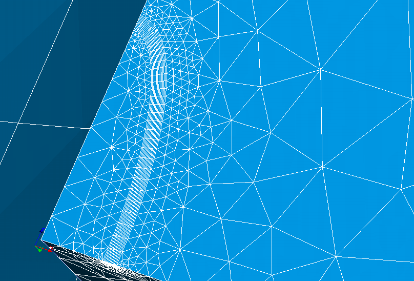
Figure 1.1-2: Defect geometry
The tube has a length of 2,000 mm, a thickness of 60 mm, and an internal radius of 270 mm.
The defect is 7.5 mm deep and 22.5 mm long.
1.2. Material properties#
A rational traction curve of the Ramberg-Osgood type is used.
\(\frac{ϵ}{{ϵ}_{0}}=\frac{\sigma }{{\sigma }_{0}}+\alpha \mathrm{.}{(\frac{\sigma }{{\sigma }_{0}})}^{n}\), with \({ϵ}_{0}=\frac{{\sigma }_{0}}{E}\)
Where:
\(n=6\)
\(\alpha =1\)
\({\sigma }_{0}=163\mathit{MPa}\)
\(E=174700\mathit{MPa}\)
\(\nu \mathrm{=}0.3\)
The law of material behavior is elasto-plastic (” VMIS_ISOT_TRAC “)
Below is its traction curve.
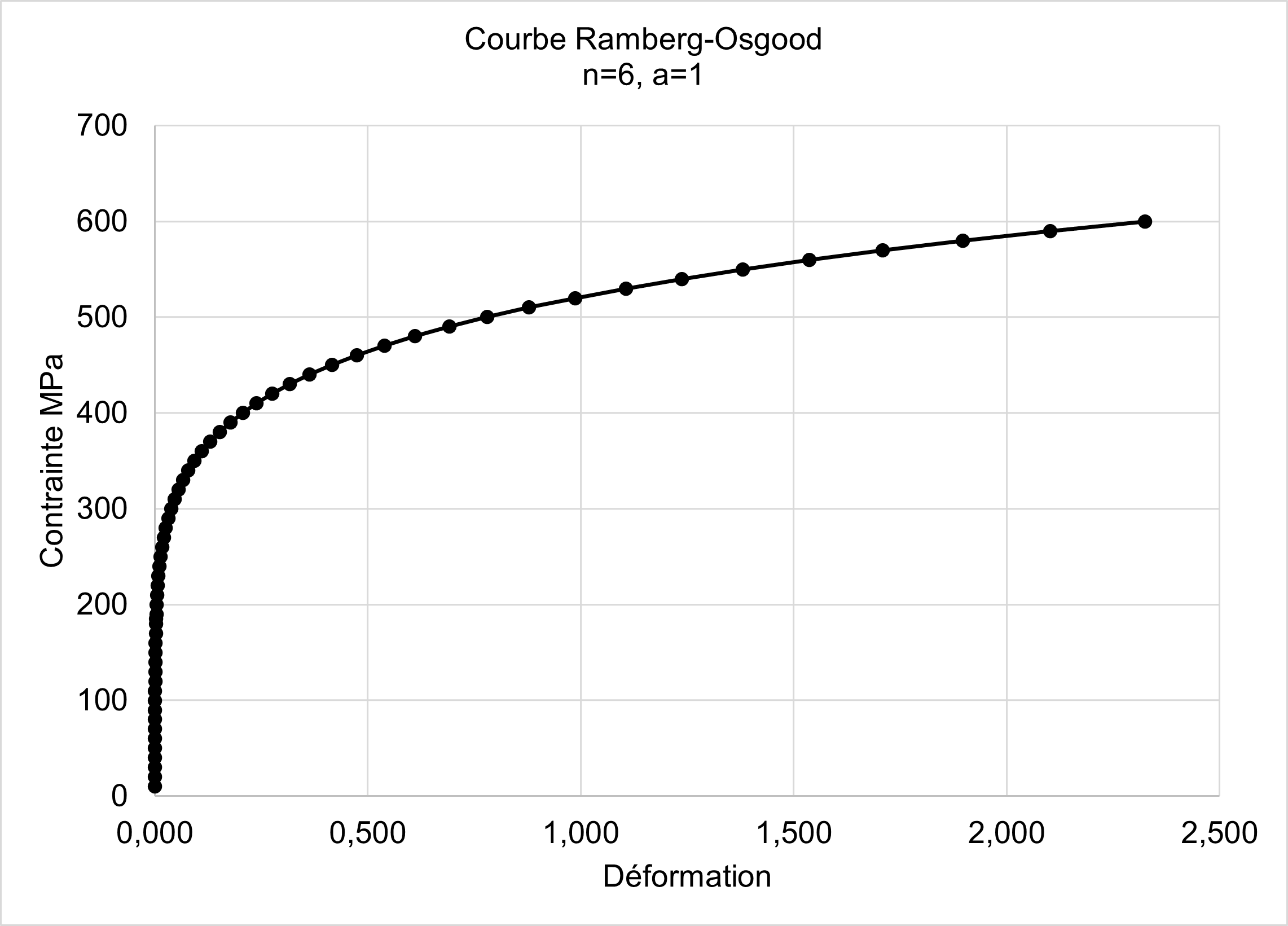
Figure 1.2-1: Ramberg-Osgood traction curve n=6, a=1 provided by [bib1].
1.3. Boundary conditions and loads#
Symmetry with respect to the 2 main planes:
\({U}_{Y}=0.\) in the \(Y=0\) plan.
\({U}_{Z}=0.\) in the \(Z=0.\) plane out of the crack
Rigid mode on the \(X\) axis.
Average \({U}_{X}\) in nodes NODE_CENTRE_FISS_T and NODE_CENTRE_FISS_TM is zero.
The loading conditions are applied in two steps:
A pressure load \(P\) is gradually applied to the inner pipe wall.
A tensile load \(\text{EFFET\_FOND}\) at the end of the pipe is also applied to model the background effect.
\(\text{EFFET\_FOND}=P\frac{{R}_{\text{int}}^{2}}{{R}_{\text{ext}}^{2}-{R}_{\text{int}}^{2}}\)
Until maximum pressure \(P=36.97\mathit{MPa}\)
By staying with a maximum pressure applied to the pipe, a next bending moment \(M\) (\(-Y\)) applying pressure to open the semi-elliptical defect is applied progressively until \(M=-5989.460\mathit{kNm}\).
It is applied to the end of the tube via a linear distribution following \(x\) of axial stresses \({\sigma }_{\mathit{zz}}\)
\({\sigma }_{\mathit{zz}}=\frac{Mx}{I}\) in the \(Z=2000\mathit{mm}\) plan
where \(I\) is the squared moment of bending. \(I=\pi \frac{({R}_{\text{ext}}^{4}-{R}_{\text{int}}^{4})}{4}\)
Below is a figure with the pipe loading path given by [bib1].
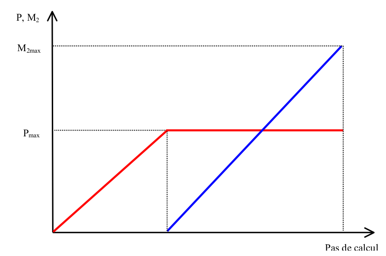
Figure 1.3-1: load path provided by [bib1].