1. Reference problem#
1.1. Geometry#
The test is carried out on the hardware point, using the SIMU_POINT_MAT command.
1.2. Material properties#
Isotropic elasticity (keyword ELAS_FO ) |
Eigencreep: properties of Kelvin chains (keyword **** BETON_GRANGER ****) ** |
|
\(E=30000\mathit{MPa}\) \(\nu =\mathrm{0,2}\) \(\alpha ={10}^{-5}\) |
\({J}_{1}=\mathrm{3,226}{10}^{-5}{\mathrm{MPa}}^{\text{–1}}\) \({J}_{2}=\mathrm{2,6}\cdot {10}^{-7}{\mathit{MPa}}^{–1}\) \({J}_{3}=\mathrm{2,7}\cdot {10}^{-6}{\mathit{MPa}}^{–1}\) \({J}_{4}=\mathrm{2,71}\cdot {10}^{-6}{\mathit{MPa}}^{–1}\) \({J}_{5}=\mathrm{8,08}\cdot {10}^{-6}{\mathit{MPa}}^{–1}\) \({J}_{6}=\mathrm{1,808}\cdot {10}^{-5}{\mathit{MPa}}^{–1}\) \({J}_{7}=\mathrm{1,901}\cdot {10}^{-5}{\mathit{MPa}}^{–1}\) \({J}_{8}=\mathrm{1,139}\cdot {10}^{-5}{\mathit{MPa}}^{–1}\) |
\({\tau }_{1}=2\cdot {10}^{-3}\text{jours}\) \({\tau }_{2}=2\cdot {10}^{-2}\text{jours}\) \({\tau }_{3}=2\cdot {10}^{-1}\text{jours}\) \({\tau }_{4}=2\text{jours}\) \({\tau }_{5}=2\cdot 10\text{jours}\) \({\tau }_{6}=2\cdot {10}^{2}\text{jours}\) \({\tau }_{7}=2\cdot {10}^{3}\text{jours}\) \({\tau }_{8}=2\cdot {10}^{4}\text{jours}\) |
Aging function (keyword V_ BETON_GRANGER ) |
||
\(k({t}_{c})=\frac{{\text{28}}^{\mathrm{0,2}}+\mathrm{0,1}}{{t}_{c}^{\mathrm{0,2}}+\mathrm{0,1}}\) |
||
Table 1.2-1
The desorption function (to be filled in under the keyword ELAS_FO) describes the appearance of the relative humidity \(h\) as a function of the water content \(C\) (which corresponds to the Code_Aster control variable SECH).
For modeling A, this function is linear if \(50\mathit{kg}/{m}^{3}\le C\le 100\mathit{kg}/{m}^{3}\) and constant outside these limits; humidity varies between the initial value \({h}_{0}=1\) and the final value \({h}_{f}=\mathrm{0,5}\) and, as shown in the.
For B modeling, it is constant and equal to \(h=1\text{(ou 100\% )}\)
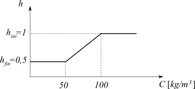
Figure 1.2-1
1.3. Boundary conditions and loads#
Mechanical limit conditions: uniaxial traction. The constraint imposed (component SIZZ) is equal to \({\sigma }_{\mathit{zz}}={\sigma }_{0}=10\mathit{MPa}\). Charging is maintained for \(1\) years.
Temperature: a constant temperature of \(T=20°C\) is uniformly imposed on the structure, equal to the reference temperature. As a result, thermal shrinkage is zero.
Water Content:
For modeling A, this function has a linear appearance. It is worth \({C}_{0}=100\) at the initial time \({t}_{0}=0\) and \({C}_{f}=50\) at the final time \({t}_{f}=365\) days.
For B modeling, it is constant and equal to \(h={h}_{0}=1\text{(ou 100\% )}\)