1. Reference problem#
1.1. Theoretical framework#
The usual buckling criterion results in a sign check of the smallest eigenvalue of the tangent matrix \(K\delta u=\mu \delta u\). If \(\mu \le 0\) the solution to the mechanical problem is no longer unique.
For mixed formulations, the natural modes associated with the presence of Lagrange coefficients must be eliminated. This brings us back to a problem with natural modes under constraint.
\(K(\begin{array}{}\delta u\\ \delta \lambda \end{array})=\mu (\begin{array}{}\delta u\\ 0\end{array})\) is the new buckling criterion for mixed modeling.
In case GRAD_VARI the criterion is even more restrictive, because it is also necessary to take into account the law of behavior to obtain physical modes. This should be able to be generalized to other types of models. The criterion is then written as a generalized eigenvalue problem:
\(K(\begin{array}{}\delta u\\ \delta \alpha \\ \delta \lambda \end{array})=\mu (\begin{array}{}\delta u\\ 0\\ 0\end{array})\) new buckling criterion for GRAD_VARI modeling.
This provides us with two equality constraints in the search for the mode on the go. The first allows us to verify the law of behavior of the material and the second the equality of the disturbances of the damage at the nodes with that calculated locally at the Gauss points.
We validate the new buckling criterion by making a comparison between the smallest modes of formulation GRAD_VARI and those of local modeling in the case of a homogeneous study.
Note:
Technically in order to achieve this, the new commands RIGI_GEOM and DDL_EXCLUS have been added to the CRIT_STAB operator. In this specific case, they are used in the following way:
CRIT_STAB = _F (RIGI_GEOM = “NON”, #*Needed to call then* DDL_EXCLUS
DDL_EXCLUS = (“VARI”, “LAG_GV”))
1.2. Geometry#

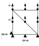
Figure 1: Representation of the problem in two quadratic cells
1.3. Material properties#
Law of damage: material ENDO_FRAGILE
Elastic characteristics:
\(E=3\cdot {10}^{4}\text{Pa}\)
\(\nu =0.25\)
Characteristics related to the law of damage:
Elastic limit: \({\sigma }^{Y}=3.0\text{Pa}\)
Softening slope: \({E}^{T}=-1.95\cdot {10}^{3}\text{Pa}\)
Non-local characteristics: \({L}_{c}=1.0\); \(r=100.\)
1.4. Boundary conditions and loads#
Embed: Zero imposed displacements \(\mathrm{DY}=0.\) on the bottom horizontal edge (\(y=0.\)) and \(\mathrm{DX}=0.\) on the extreme left node (\(x=y=0.\)). See figure 1.
Loading 1: Imposed displacement \({U}_{1}\) on the top horizontal edge (\(y=1.\)):
\(\mathrm{DY}={2.10}^{-6}\text{t}\)
Loading 2: Imposed displacement \({U}_{2}\) on all \(y=0.5\) coordinate nodes:
\(\mathrm{DY}={1.10}^{-6}\text{t}\)