2. Modeling A#
The analysis is static with linear elastic behavior, the model used is of type C_ PLAN.
2.1. Optimization settings#
The basic structure was built considering the following parameters:
No mesh for grid interpolation in the X direction → PAS_X = 0.05m
No mesh for grid interpolation in Y direction → PAS_Y = 0.05m
Maximum element length → LONGUEUR_MAX = 2m
Minimum distance between stress peaks → TOLE_BASE = 0.01
The optimization of the basic geometry according to the SECTION type scheme is carried out with the following parameters:
Maximum number of iterations MAXITER = 200
Optimization convergence threshold RESI_RELA_SECTION = 0.000001
Maximum section evolution rate per iteration CRIT_SECTION = 50%
Minimum element section SECTION_MINI = 10-10 m2
The optimization according to the TOPO scheme (optimization of the sections plus topological optimization) is carried out with the following additional parameters:
Optimization convergence threshold RESI_RELA_TOPO = 0.00001
Maximum element elimination rate CRIT_ELIM = 0.5
Control of pseudo-random variables INIT_ALEA = 2
2.2. Basic structure built#
The basic structure is thus built within the macro command CALC_BT based on the results of the 2D modeling and considering the parameters defined in the previous section.
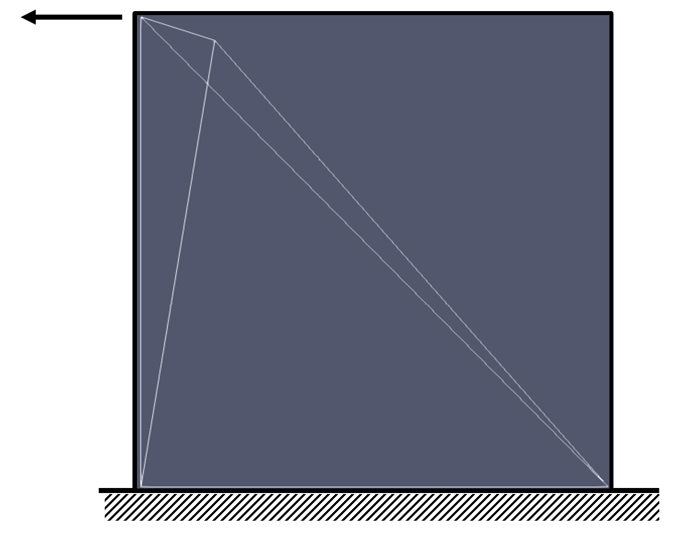
Picture 2.2-1
2.3. Optimization SCHEMA = “SECTION”#
The following Figure shows the forces distributed among the elements of the structure at the end of the optimization process according to diagram SECTION (optimization of sections only).
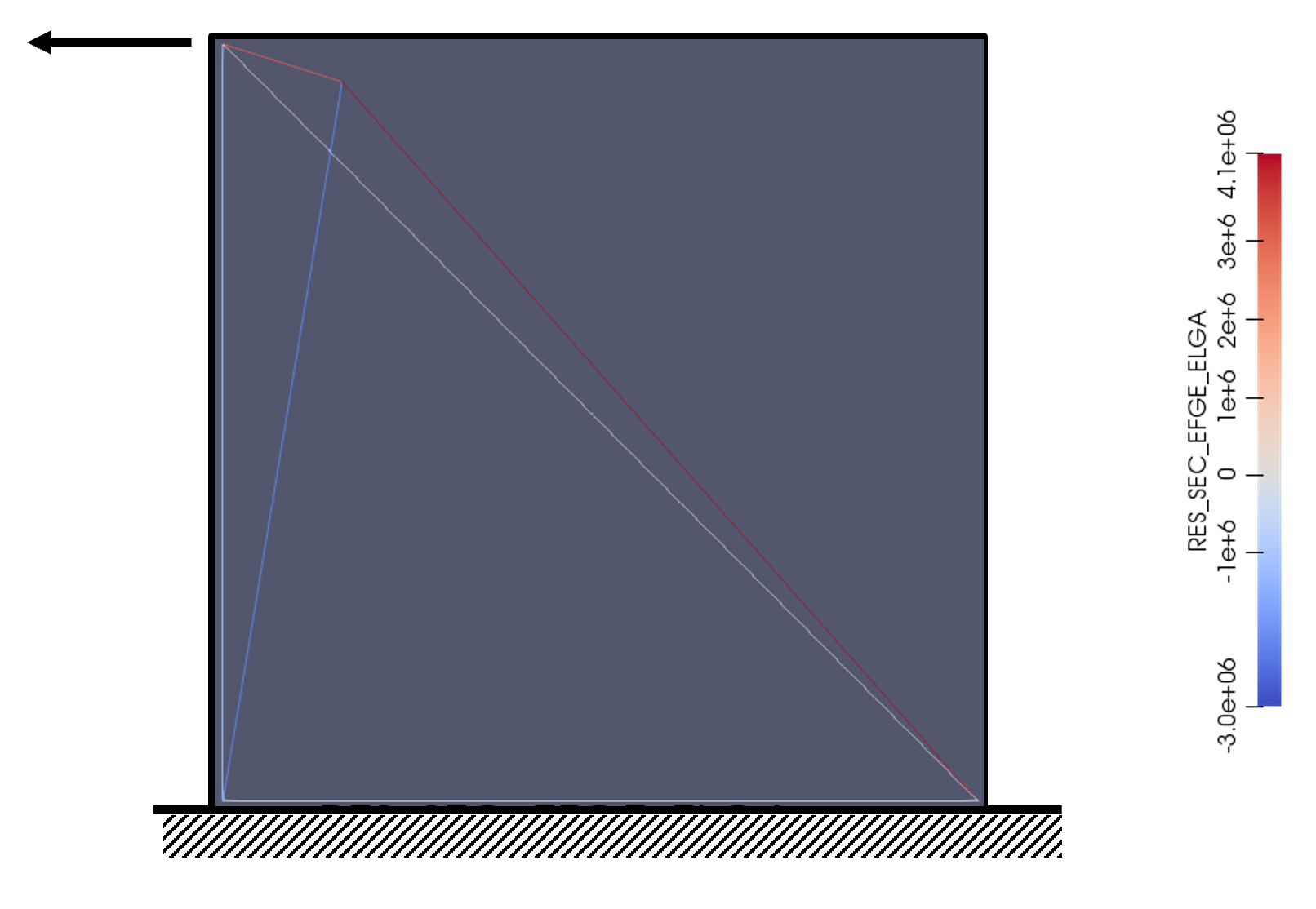
Picture 2.3-1
Table 2.2.2-1 shows the results of the optimization procedure. In order to facilitate the comparison of results, the numbering of the items (first column) has been changed manually.
COORD XI |
COORD YI |
COORD XJ |
COORD YJ |
TYPE |
N |
N |
A |
L |
ENEL_ELEM |
||||
B1 |
0.00 |
0.00 |
0.00 |
0.15 |
0.15 |
0.95 |
|
-2.18E+06 |
6.24E-02 |
0.96 |
0.96 |
3.50E+04 |
|
B3 |
0.00 |
0.00 |
0.00 |
0.95 |
0.95 |
0.00 |
|
0.00E+00 |
1.00E-06 |
0.95 |
0.95 |
0.00E+00 |
|
B2 |
0.00 |
0.00 |
0.00 |
0.00 |
0.00 |
1.00 |
|
-1.00E+06 |
2.86E-02 |
1.00 |
1.00 |
1.67E+04 |
|
T1 |
0.15 |
0.95 |
0.95 |
0.95 |
0.95 |
0.00 |
|
4.13E+06 |
8,26E-03 |
1.24 |
1.24 |
1.24 |
1.22E+05 |
T2 |
0.15 |
0.95 |
0.95 |
0.00 |
0.00 |
1.00 |
|
3.16E+06 |
6.32E-03 |
0.16 |
0.16 |
1.16 |
1.19E+04 |
T3 |
0.95 |
0.00 |
0.00 |
0.00 |
0.00 |
1.00 |
|
5.80E-02 |
1.00E-06 |
1.38 |
1.38 |
2.21E-07 |
Table 2.3-1: Optimized structure: C_ PLAN, SCHEMA = SECTION
2.4. Optimization SCHEMA = “TOPO”#
The following Figure and Table show the distribution of forces in the elements of the structure at the last iteration. As if in the results of section 2.2.2, the numbering of the items (first column of the Table) was manually changed.
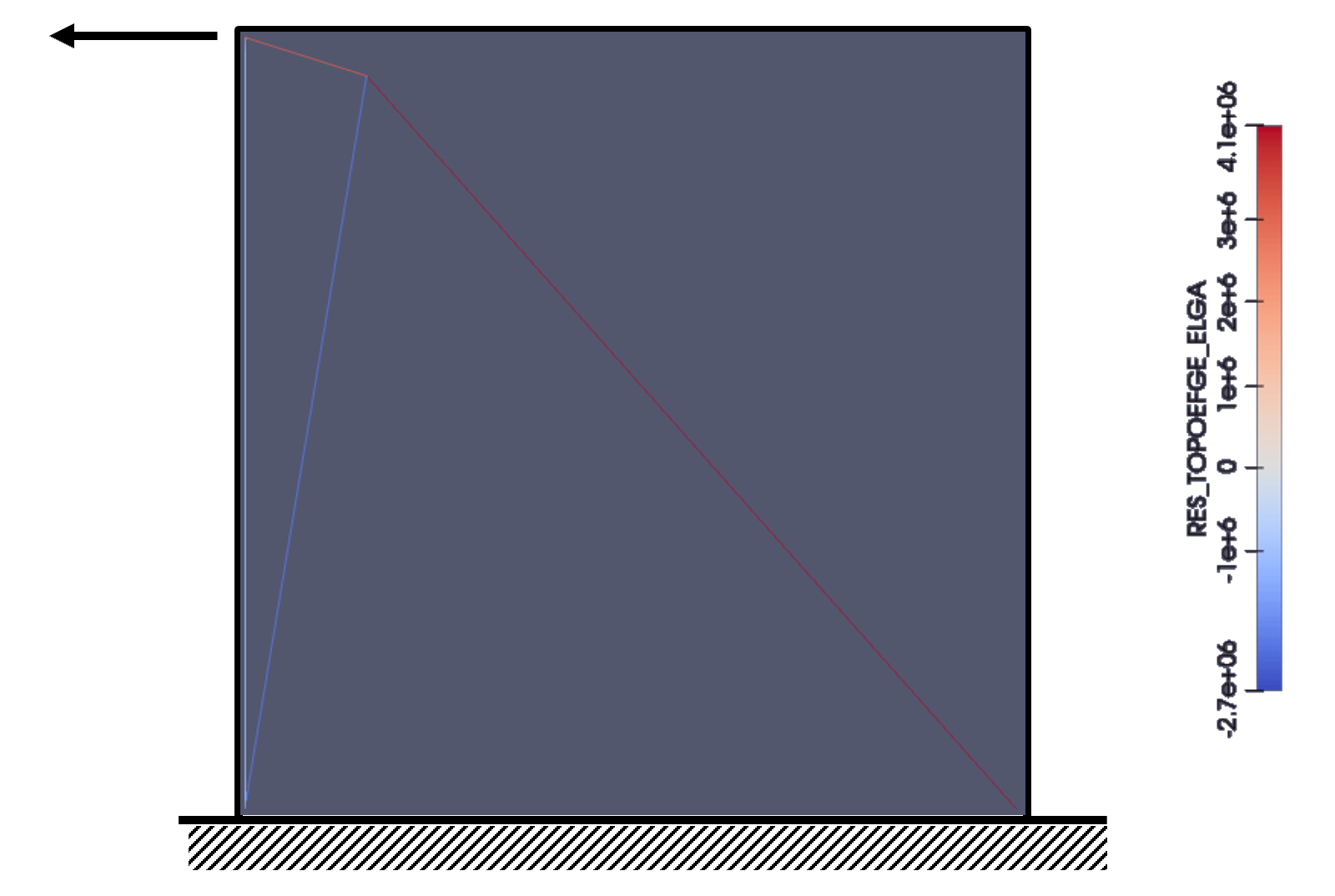
Picture 2.4-1
# |
COORD XI |
COORD YI |
COORD XJ |
COORD YJ |
TYPE |
N |
N |
A |
L |
ENEL_ELEM |
|||
B1 |
0.00 |
0.00 |
0.00 |
0.15 |
0.15 |
0.95 |
|
-2.18E+06 |
6.24E-02 |
0.96 |
0.96 |
3.50E+04 |
|
B2 |
0.00 |
0.00 |
0.00 |
0.00 |
0.00 |
1.00 |
|
-1.00E+06 |
2.86E-02 |
1.00 |
1.00 |
1.67E+04 |
|
T1 |
0.15 |
0.95 |
0.95 |
0.95 |
0.95 |
0.00 |
|
4.13E+06 |
8,26E-03 |
1.24 |
1.24 |
1.24 |
1.22E+05 |
T2 |
0.15 |
0.95 |
0.95 |
0.00 |
0.00 |
1.00 |
|
3.16E+06 |
6.32E-03 |
0.16 |
0.16 |
1.16 |
1.19E+04 |
Table 2.4-1 ****: ****Optimized structure:C_ PLAN, SCHEMA = TOPO **