2. Benchmark solution#
2.1. Method for calculating the continuous problem#

Figure 2.1-a : Diagram of the plate and springs after loading.
Solving the problem consists in calculating the vertical displacements of the corners of the plate and the position of the detachment point with respect to the spring belt.
The equilibrium equations are as follows:
Effort resulting from loading:
\(\mathrm{Fp}=\underset{s}{\iint }\mathrm{P.ds}=\mathrm{a.p.}\frac{{b}^{3}}{3}\) [2.1-1]
Moment resulting from point \(A\) due to loading:
\({\mathrm{Mp}}_{A}=\underset{s}{\iint }\mathrm{P.y.ds}=\mathrm{a.p.}\frac{{b}^{4}}{12}\) [2.1-2]
The plate is considered to be rigid, its displacement is in the form \(z(y)={U}_{a}(1-\frac{y}{{y}_{0}})\). With \({U}_{a}\) the vertical displacement of the point \(A\) and \({y}_{0}\) the position of the detachment.
Spring reaction force:
\(\mathrm{Fr}=\underset{s}{\iint }\frac{K}{\mathrm{a.b}}{U}_{a}(1-\frac{y}{{y}_{0}})\mathrm{ds}=K{U}_{a}\frac{{y}_{0}}{2b}\) [2.1-3]
Reaction moment of the springs at point \(A\):
\({\mathrm{Mr}}_{A}=\underset{s}{\iint }\frac{K}{ab}{U}_{a}(1-\frac{y}{{y}_{0}})y\mathrm{ds}=K{U}_{a}\frac{{y}_{0}^{2}}{6b}\) [2.1-4]
Solving the equations,,, (balance of efforts and moments) gives the following result:
\({y}_{0}=\frac{3b}{4}{U}_{a}=-\frac{8pa{b}^{3}}{9K}\) we deduce \({U}_{b}=-\frac{{U}_{a}}{3}\)
2.2. Method for calculating the discretized problem#
In this analysis the spring mat is no longer considered to be continuous. The springs are evenly distributed. As before, the vertical displacements of the corners of the plate and the position of the separation line with respect to the spring belt will be calculated.
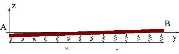
Figure 2.2-a : Diagram of the plate and springs after loading.
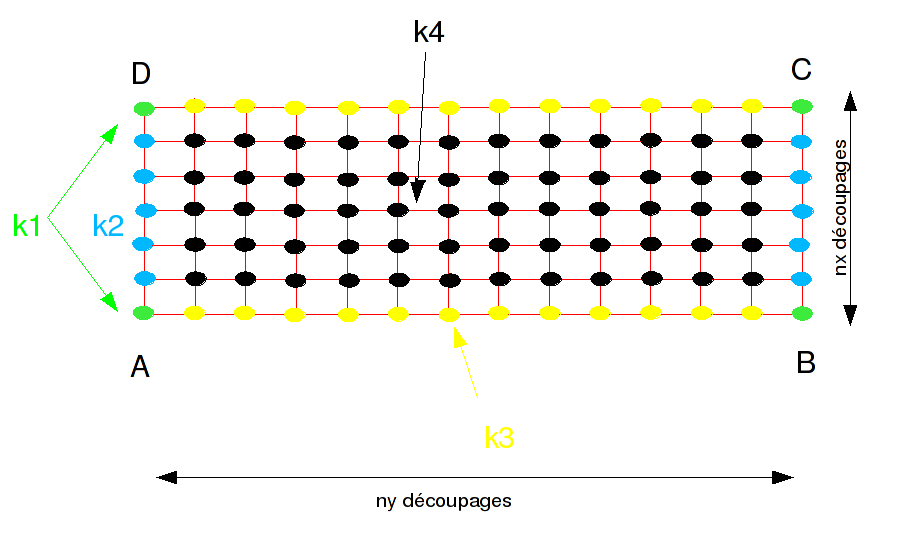
Figure 2.2-b : Discretization of the plate in the plane \((x,y)\) .
The figure above identifies the springs according to their stiffness. This stiffness is calculated by option RIGI_PARA_SOL of the AFFE_CARA_ELEM command. The assignment of values is based on the area of the area they affect. If \(K\) is the overall stiffness of the spring pad, we therefore have:
\(\text{k4}=\frac{\text{K}}{\mathrm{nx}\mathrm{ny}}\text{k2}=\text{k3}=\frac{\text{k4}}{2}=\frac{\text{K}}{2\mathrm{nx}\mathrm{ny}}\text{k1}=\frac{\text{k4}}{4}=\frac{\text{K}}{4\mathrm{nx}\mathrm{ny}}\) [2.2-1]
The equilibrium equations are as follows:
Spring reaction force:
\({\mathit{Fr}}_{(j)}={U}_{a}\cdot \left[{K}_{x}^{\text{'}}+{K}_{x}^{\text{'}\text{'}}\cdot \sum _{j=1}^{n}\left(1-j\frac{b}{\mathit{ny}{y}_{0}}\right)\right]\) [2.2-2]
Spring reaction moment along line \(\mathrm{AB}\):
\({\mathrm{Mr}}_{(j)}={U}_{a}\cdot {K}_{x}^{\text{'}\text{'}}\cdot \sum _{j=1}^{n}(1-j\frac{b}{\mathrm{ny}{y}_{0}})\cdot j\frac{b}{\mathrm{ny}}\) [2.2-3]
with \({K}_{x}^{\text{'}}=(2\text{k1}+\text{k2}(\mathrm{nx}-1)){K}_{x}^{"}=(2\text{k3}+\text{k4}(\mathrm{nx}-1))\)
\(n\frac{b}{\mathrm{ny}}\le {y}_{0}\le (n+1)\frac{b}{\mathrm{ny}}\)
Solving the equations (balance of efforts and moments) gives the solution of the balance:
\({U}_{a}=\frac{pa{b}^{3}\mathrm{ny}(3\mathrm{ny}-8n-4)}{6K(1+n+{n}^{2})}{y}_{0}=\frac{bn(1+n)(3\mathrm{ny}-8n-4)}{3\mathrm{ny}(\mathrm{ny}+2n(\mathrm{ny}-2)-4{n}^{2})}\) [2.2-4]
where \(n\) and \({y}_{0}\) must meet the following conditions:
\(\mathrm{n.}\frac{b}{\mathrm{ny}}\le {y}_{0}\le (n+1)\frac{b}{\mathrm{ny}}\) \(0\le {y}_{0}\le b\) \(n\) integer
2.3. Reference quantities and results#
The quantities tested will be the vertical displacements at the 4 corners of the plate.
2.4. Uncertainties about the solution#
None, the solution is analytical.