2. Benchmark solution#
We consider one of the laws of behavior with a damage gradient [R5.04.01] whose free energy density is in the following form:
\(\Phi (\varepsilon ,a)\mathrm{=}A(a)w(\varepsilon )+\omega (a)+c\mathrm{/}2{(\mathrm{\nabla }a)}^{2}\), where \(0\le a\le 1\) refers to the damage variable and \(w(\varepsilon )\) refers to the elastic deformation energy. For law ENDO_SCALAIRE, \(\omega (a)=\mathrm{ka}\) and the damage prefactor is written as \(A(a)\mathrm{=}{(\frac{1\mathrm{-}a}{1+\gamma a})}^{2}\). The solution then depends on three material parameters \(\gamma\), \(c\), and \(k\) (see [R5.03.18]).
In the general case, two partial differential equations need to be solved: the equilibrium equation (\(\delta \Phi (\varepsilon ,a)/\delta \varepsilon =0\)) and the behavior equation \(\delta \Phi (\varepsilon ,a)/\delta a=0\). Obtaining an analytical solution is generally difficult, even for one-dimensional structures. To validate this model, however, we focus on a simpler problem for which the equilibrium equation does not need to be solved, i.e. the field of displacement is fixed everywhere. The behavior equation is then controlled by the elastic deformation energy \(w\) known at every point in space. In this simplified case, the semi-analytical solution is obtained by a numerical integration of a differential equation with the initial Cauchy conditions.
As for law ENDO_FISS_EXP, it is completely equivalent to law ENDO_SCALAIRE in a uniaxial traction situation. The analytical solution is therefore identical to that for ENDO_SCALAIRE.
2.1. Characterization of the solution#
More precisely, a bar is considered, one part of which is required to remain without deformation while the other is subject to homogeneous deformation. The damage boundary layer that develops at the interface of these two zones is then studied. The differential behavior equation is as follows in the areas where the criterion is met, that is to say where the damage evolves:
\(c\frac{{\mathrm{\partial }}^{2}a}{\mathrm{\partial }{x}^{2}}\mathrm{-}\frac{\mathrm{\partial }A}{\mathrm{\partial }a}w\mathrm{-}k\mathrm{=}0\), where \(\frac{\mathrm{\partial }A}{\mathrm{\partial }a}(a)\mathrm{=}\mathrm{-}2(1+\gamma )\frac{(1\mathrm{-}a)}{{(1+\gamma a)}^{3}}\), eq 2.1-1
where \(x\) refers to the space variable.
The elastic deformation energy \(w\) is known in each of the two parts of the bar: \(w=0\) on the left and \(w({\varepsilon }_{0})=\mathrm{const}\) on the right. The solution is given by a differentiable continuous function \(a\in {C}^{1}(-{L}_{\mathrm{0,}}{L}_{1})\).
There are three following boundary conditions:
\(\frac{da}{dx}(-{L}_{0})=\frac{da}{dx}({L}_{1})=0\) and \(a(-{L}_{0})=0\) eq 2.1-2
as well as two interface conditions:
\({\left[\mid a\mid \right]}_{x=0}=0{\left[∣\frac{da}{dx}∣\right]}_{x=0}=0\) eq 2.1-3
So in total, we have five boundary conditions for five unknowns. Despite this fact, the problem is « poorly posed » in order to be able to be solved numerically, because the boundary conditions are defined at different points in space. We then proceed to identify the unknowns using the boundary conditions and finally obtain an ordinary differential equation of the Cauchy-Lipschitz type.
2.2. Solving the problem in the unloaded area#
It is assumed that the left end of bar \(x=-{L}_{0}\) is located far enough from the \(x=0\) interface for the hypothesis of a finite length boundary layer in the unloaded area to remain valid. Let us then note \({b}_{0}>0\) the length (a priori dependent on the level of deformation \({\varepsilon }_{0}\) in the loaded zone) over which this boundary layer develops.
In part \(x\in \left[{L}_{0},-{b}_{0}\right]\) the damage does not evolve and remains zero:
\(a(x)=0\) out of \(\left[-{L}_{0},-{b}_{0}\right]\) eq 2.2-1
In part \(x\in \left[-{b}_{0}\mathrm{,0}\right]\), the criterion is reached and the damage field evolves according to equation [éq 2.1-1], which is considerably simplified in this part of the bar since the elastic deformation energy is zero there:
\(c\frac{{d}^{2}a}{{\mathrm{dx}}^{2}}=k\) out of \(\left[-{b}_{0}\mathrm{,0}\right]\) eq 2.2-2
By definition of \({b}_{0}\), we have the following conditions:
\(a(-{b}_{0})=0\) and \(\frac{\mathrm{da}}{\mathrm{dx}}(-{b}_{0})=0\) eq 2.2-4
We can then express the damage variable analytically by integrating [éq 2.2-2]:
\(a(x)=\frac{k}{\mathrm{2c}}{(x+{b}_{0})}^{2}\) out of \(\left[-{b}_{0}\mathrm{,0}\right]\) eq 2.2-5
We then know the values of the damage and its derivative at the interface \(x=0\), as a function of the unknown \({b}_{0}\):
\(a({0}^{-})=\frac{{\mathrm{kb}}_{0}^{2}}{2c}\) and \(a\text{'}({0}^{-})=\frac{{\mathrm{kb}}_{0}}{c}\) eq 2.2-6
and the damage at the interface \({a}_{0}\) being strictly between \(0\) and \(1\), the following frame of length \({b}_{0}\) is deduced:
\(0<{a}_{0}<1\Rightarrow 0<{b}_{0}<\sqrt{\frac{\mathrm{2c}}{k}}\) eq 2.2-7
It is therefore sufficient to take the left part of the bar longer than \(\sqrt{\mathrm{2c}/k}\) to be sure to have the damage profile confined to the left.
2.3. Solving the problem in the loaded area#
This part of the bar sees a homogeneous deformation \({\varepsilon }_{0}>0\) associated with an elastic deformation energy \({w}_{0}\). In this zone, the boundary layer is no longer bounded and extends asymptotically towards the homogeneous response. We will therefore assume that the right end of the bar \(x={L}_{1}\) is located far enough from the \(x=0\) interface to be able to approximate a zero derivative for the damage field « at infinity ». In the vicinity of the right end of the bar, the behavior equation [éq 2.1-1] is then reduced to:
\(\frac{-\partial A}{\partial a}({a}_{\infty }){w}_{0}=k\) eq 2.3-1
where \({a}_{\infty }\) refers to the asymptotic value of the damage field. Given the expression for \(\partial A/\partial a\) (cf. [éq 2.1-1]), we can then set the load level by the only value \({a}_{\infty }\):
for \({a}_{\infty }\in \left]\mathrm{0,1}\right[,{w}_{0}=\frac{k}{2(1+\gamma )}\frac{{(1+\gamma {a}_{\infty })}^{3}}{(1-{a}_{\infty })}\) eq 2.3-2
On the other hand, the nonlinear differential equation [éq 2.1-1] can be written in the following form:
\(\frac{c}{2}2a\text{'}a\text{'}\text{'}=a\text{'}(A\text{'}(a)w-k)\) eq 2.3-3
It therefore admits a first integral:
\(\forall x\in \left[\mathrm{0,}{L}_{1}\right],{\left[\frac{c}{2}{(\frac{\mathrm{da}}{\mathrm{dx}}(s))}^{2}\right]}_{0}^{x}={\left[A(a(s))+ka(s)\right]}_{0}^{x}\) eq 2.3-4
We recall that the interface condition [éq 2.1-3] imposes a connection \({C}^{1}\) in \(x=0\), taking into account the expressions linking \(a({0}^{+})\) and \(a\text{'}({0}^{+})\) to the length \({b}_{0}\) of the boundary layer we can then write:
\({a}_{0}=a({0}^{+})=\frac{{\mathrm{kb}}_{0}^{2}}{2c}\) and \(a{\text{'}}_{0}=a\text{'}({0}^{+})=\sqrt{\frac{2k}{c}{a}_{0}}\) eq 2.3-5
In addition, the boundary conditions [éq 2.1-2] ensure the nullity of the derivative of the damage in \(x={L}_{1}\), by making the approximation \(a({L}_{1})={a}_{\infty }\), the first integral [éq 2.3-4] evaluated in \(x={L}_{1}\) amounts to:
\(A({a}_{0}){w}_{0}+k{a}_{0}-\frac{c}{2}a{\text{'}}_{0}^{2}=A({a}_{\infty }){w}_{0}+k{a}_{\infty }\) eq 2.3-6
The equation [éq 2.3-6] is simplified according to [éq 2.3-5], it is then reduced to the following quadratic trinomial of unknown \({a}_{0}\):
\((f({a}_{\infty }){\gamma }^{2}-1){a}_{0}^{2}+2(f({a}_{\infty })\gamma +1){a}_{0}+(f({a}_{\infty })-1)=0\) where \(f({a}_{\infty })=A({a}_{\infty })+\frac{k{a}_{\infty }}{{w}_{0}}\) eq 2.3-7
We therefore have a simple relationship between the loading parameter \({a}_{\infty }\) and the value \({a}_{0}\) of the damage as well as its derivative \(a{\text{'}}_{0}\) at the interface.
The resolution of the nonlinear EDO [éq 2.1-1] on \(\left[\mathrm{0,}{L}_{1}\right]\) was achieved by reducing it to a differential system of order 1, numerically integrated with a Runge-Kutta diagram at order 4 (in space). The implementation of this scheme only requires knowledge of the initial conditions \(({a}_{\mathrm{0,}}a{\text{'}}_{0})\) associated with each loading parameter \({a}_{\infty }\), which is ensured by the relationship [éq 2.3-7]
2.4. Solving the problem in the entire bar#
In order to calculate the reference solution over the entire bar, the following diagram is adopted:
choice of a loading parameter \({a}_{\infty }\in \left]\mathrm{0,1}\right[\)
Resolution in the loaded part:
determination with [éq 2.3-2] of the associated elastic deformation energy \({w}_{0}\)
determination with [éq 2.3-7] of the set of boundary conditions \(({a}_{\mathrm{0,}}a{\text{'}}_{0})\)
numerical integration with a Runge-Kutta diagram in order 4
Resolution in the unloaded part:
determination with [éq 2.3-7] and [éq 2.3-5] of the size \({b}_{0}\) of the boundary layer in the unloaded area
obtained with [éq 2.2-5] the analytical field \(a(x)\) in this zone
2.5. Digital application#
For elasticity, work-hardening and the non-local parameter, the following characteristics are adopted:
\(\begin{array}{cc}E={3.10}^{4}\mathrm{MPa}& {\sigma }^{y}=3.\mathrm{MPa}\\ \nu =0.& \gamma =4.\end{array}c=1.875N\) eq 2.5-1
These choices lead to a threshold elastic deformation energy:
\({w}_{y}=1.5{10}^{-4}\mathrm{MPa}\) eq 2.5-2
2.6. Benchmark results#
The reference solution is obtained by taking a bar of length \(-{L}_{0}=-125\mathrm{mm}\) and \({L}_{1}=250\mathrm{mm}\). The damage field value \(a\) is examined for three loading levels and in two locations, one in the unloaded area and the other in the loaded area.
\({\varepsilon }_{0}\) |
|
\(a(x=-7.5\mathrm{mm})\) |
|
|
2.70000000000000E-04 |
1.09350000000000E-003 |
1.93274688119012E-02 |
1.4184667575324338E-01 |
|
7,34846922834953E-04 |
8,10053999999999E-003 |
1,39107889370765E-01 |
3,80008828953E-04 |
3,8000882828951670E-01 |
1,10464444958548E-02 |
1,83060308787201E+000 |
6,14240950943351E-01 |
9,77312427816067E-01 |
9,77312427816067E-01 |
Table 2.6-1 - Benchmark Results
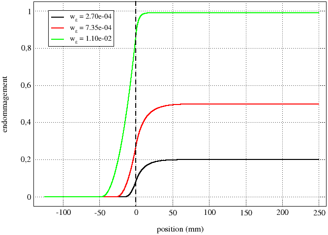
Figure 2.6-1: Damage profile for the reference solution