1. Reference problem#
1.1. Geometry#
The geometry used in this test case is a reinforced concrete plate with a thickness of \(e\mathrm{=}0.1\text{m}\) and a trapezoidal shape.
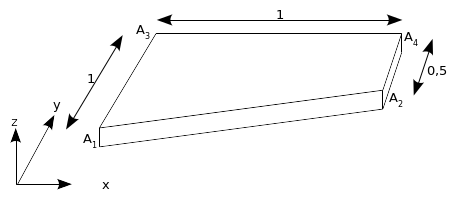
Figure 1.1-a : Geometry studied
The characteristics of the reinforced concrete section are:
Upper sheet: section per linear meter following \(x\) and \(y\) \(=5.65{10}^{-4}{m}^{\mathrm{²}}/\mathrm{ml}\); eccentricity with respect to the following mean sheet \(x\) and \(y\): \(+0.0475m\) (i.e. 95% of the thickness),
Lower sheet: section per linear meter following \(x\) and \(y\) \(=5.65{10}^{-4}{m}^{\mathrm{²}}/\mathrm{ml}\); eccentricity with respect to the following mean sheet \(x\) and \(y\): \(-0.0475m\) (i.e. 95% of the thickness),
Prestress cables: section per linear meter following \(x=4.56{10}^{-3}{m}^{\mathrm{²}}/\mathrm{ml}\) and \(y=1.32{10}^{-2}{m}^{\mathrm{²}}/\mathrm{ml}\); no eccentricity compared to the middle sheet; pretension following \(x\) and \(y\) \(=-3\mathrm{MN}\),
Liner: the thickness of the liner is \(6\mathrm{mm}\) and is positioned on the underside.
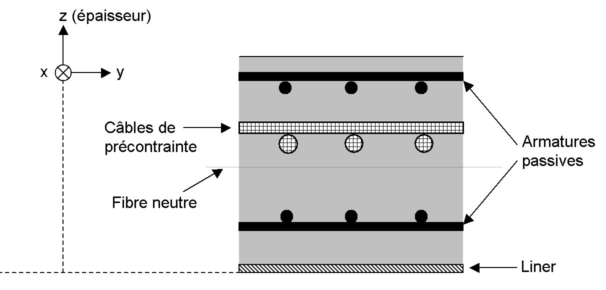
Figure 1.1-b : Reinforced concrete plate section
1.2. Material properties#
The characteristics of the various materials for modeling GLRC_DAMAGE are summarized in the following table.
Material |
Young’s Module \(\mathrm{MPa}\) |
Fish Coefficient |
Density \(\mathrm{kg}/{m}^{3}\) |
Work hardening slope |
Elastic tensile limit |
Elastic tensile limit \(\mathrm{MPa}\) |
Elastic compression limit \(\mathrm{MPa}\) |
|
Concrete |
30,000. |
0.2 |
2500 |
0 |
0 |
5 |
-35 |
|
Reinforcement steel |
200000 |
0 |
3000 |
-3000 |
-3000 |
|||
Liner steel and pretension cables |
200000 |
200000 |
0 |
500 |
-500 |
To complete the law of behavior GLRC_DAMAGE, it is necessary to define the globalized parameters of homogenized law.
Settings |
Values |
\(\mathit{Gamma}\) |
|
\(\mathit{QP1}\) |
|
\(\mathit{QP2}\) |
|
\({C}_{N}\) |
|
\({C}_{M}\) |
|

Figure 1.2-a : Moment—curvature curve of the behavior of a reinforced concrete plate under bending.
The material characteristics for modeling GLRC_DM are summarized in the following table.
Settings |
Values |
\({E}_{\mathit{éq}}^{m}\) |
|
\({\nu }_{m}\) |
|
\({E}_{\mathit{éq}}^{f}\) |
|
\({\nu }_{f}\) |
|
\({\gamma }_{\mathit{mt}}\) |
|
\({\gamma }_{f}\) |
|
\({N}_{D}\) |
|
\({M}_{D}\) |
|
1.3. Boundary conditions and loads#
On corner \(\mathrm{A1}\) of the plate, we embed the movements \({u}_{x}={u}_{y}={u}_{z}=0\), as well as the rotations \({\theta }_{x}\mathrm{=}{\theta }_{y}\mathrm{=}{\theta }_{z}\mathrm{=}0\). Travel is blocked following \(x\) and \(z\) on the sides \(\mathrm{A1A3}\) and \(\mathrm{A2A4}\). Pressure is applied to the entire slab in the direction \((0.0\mathrm{,0}.0\mathrm{,1}\mathrm{,0})\) and is equal to \({F}_{0}=20.{10}^{7}N\) for modeling A. For models B and C, a nodal force is applied to the whole slab \(1500N\). This force is applied progressively by following the multiplier function shown in the following figure.
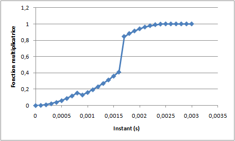
Figure 1.3-a: Load multiplier function for B and C models
1.4. Initial conditions#
In the initial state, displacements and speeds are zero everywhere.