1. Reference problem#
1.1. Geometry#
Structure \(\mathrm{2d}\) is a unitary square (\(\mathit{LX}\mathrm{=}1m\), \(\mathit{LY}\mathrm{=}1m\)), with a right crack leading to the right, located halfway up. (Figure). We call the left line the line in \(x\mathrm{=}0\), the right line the line in \(x\mathrm{=}\mathit{LX}\), and the bottom line the line in \(y\mathrm{=}0\).
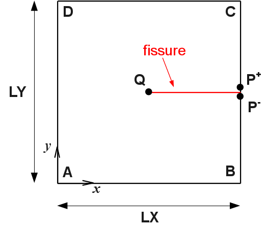
Figure 1.1-a : Geometry of the cracked square plate
Note \({P}^{\text{+}}\) the coordinate point \(\left(\mathit{LX},{\mathit{LY}}^{\text{+}}/2\right)\) (located on the upper lip), \({P}^{\text{-}}\) the coordinate point \((\mathit{LX},{\mathit{LY}}^{\text{-}}\mathrm{/}2)\) (located on the lower lip), and \(Q\) the coordinate point \(\left(\mathit{LX}/\mathrm{2,}\mathit{LY}/2\right)\) (located at the tip of the crack).
1.2. Material properties#
Thermal conductivity: \(\lambda =1{\mathit{W.m}}^{\text{-1}}\mathrm{.}{K}^{\text{-1}}\)
Calorific volume capacity: \(\rho {C}_{p}=2\mathit{J.m}-{\mathrm{3.K}}^{-1}\)
Exchange coefficient between the lips of the crack \(h=2{\mathit{W.m}}^{\text{-2}}\mathrm{.}{K}^{\text{-1}}\)
1.3. Boundary conditions and loads#
We solve the problem on the discretized time interval \(\left[0\text{.}s,1\text{.}s\right]\) in 5 equal time steps (of duration \(\Delta t=0.2s\)). We take the value by default in THER_LINEAIRE of the theta-schema parameter: \(\theta =0.57\).
On the nodes of segment \(\mathit{AB}\) (see Figure), the following temperature ramp is imposed:
to \(t=0\text{.}s\), \(\text{}\stackrel{̄}{T}{\text{}}^{\mathit{AB}}=10°C\); to \(t=1\text{.}s\), \(\text{}\stackrel{ˉ}{T}{\text{}}^{\mathit{AB}}\mathrm{=}20°C\)
On the nodes of segment \(\mathit{CD}\) (see Figure), the following temperature ramp is imposed:
to \(t=0\text{.}s\), \(\text{}\stackrel{̄}{T}{\text{}}^{\mathit{CD}}=20°C\); to \(t=1\text{.}s\), \(\text{}\stackrel{̄}{T}{\text{}}^{\mathit{CD}}=40°C\)
Finally, on the lips of the crack, a Neumann condition, such as an exchange condition, is imposed.
1.4. Initial conditions#
The initial state is determined by solving the stationary problem at \(t\mathrm{=}0\text{.}s\) (with the boundary conditions given in paragraph 1.3)