3. Modeling A#
3.1. Characteristics of modeling#
It’s a \(\mathrm{3D}\) XFEM modeling with linear elements.
This modeling demonstrates the good functioning of « estimative » criteria with linear elements. The interface is positioned such that the 1% interface readjustment threshold is reached: the interface is then modified and readjusted to the nearest nodes. This modification makes it possible to control the packaging. On the other hand, readjusting the interface significantly degrades the quality of the results for linear elements (for quadratic elements, this readjustment is removed, to replace it by algebraic pre-conditioning).
The equation for interface XFEM is: \(x+y+z+0.01=0\).
3.2. Characteristics of the mesh#
Number of knots: 125
Mesh: 64 HEXA8 type meshes
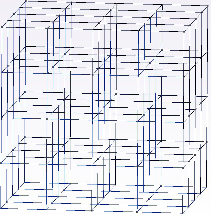
Figure 3.2-1: linear mesh
3.3. Tested sizes and results#
We test the maximum error on the displacement, in absolute value, along the interface XFEM. A list of points located on the interface is extracted, as well as the displacement field interpolated at these points.
As the displacement field is discontinuous, at each point of the interface, there are 2 analytical values of the displacement field \({U}^{\text{+}}\left(x,y,z\right)=\{{U}_{1}^{\text{+}},{U}_{2}^{\text{+}},{U}_{3}^{\text{+}}\}\) and \({U}^{\text{-}}\left(x,y,z\right)=\{{U}_{1}^{\text{-}},{U}_{2}^{\text{-}},{U}_{3}^{\text{-}}\}\). These analytical values are compared to the interpolated displacement field at each point.
In practice, in the Code_Aster to take into account the discontinuity during interpolation, each point on the interface is transformed into duplicate nodes (NP*and NM*) to which are associated displacement values \({\mathit{DX}}_{i}(\mathit{NP})\) and \({\mathit{DX}}_{i}(\mathit{NM})\).
For the « PLUS » nodes (noted NP by default in the Code_aster), the following difference table is then calculated \(\mathit{DIFF}{(\mathit{NP})}_{i}=∣{U}_{i}^{\text{+}}({x}_{\mathit{NP}},{y}_{\mathit{NP}},{z}_{\mathit{NP}})-{\mathit{DX}}_{i}(\mathit{NP})∣\);
for the nodes « MOINS » (noted NM by default in the Code_aster), the following difference table is then calculated \(\mathit{DIFF}{(\mathit{NM})}_{i}=∣{U}_{i}^{\text{-}}({x}_{\mathit{NM}},{y}_{\mathit{NM}},{z}_{\mathit{NM}})-{\mathit{DX}}_{i}(\mathit{NM})∣\).
Identification |
Reference |
Type |
% tolerance |
\(\text{DIFF}{\text{(NP)}}_{X}\) (MAX) |
0.0 |
Analytics |
0.2 |
\(\text{DIFF}{\text{(NP)}}_{Y}\) (MAX) |
0.0 |
Analytics |
0.2 |
\(\text{DIFF}{\text{(NP)}}_{Z}\) (MAX) |
0.0 |
Analytics |
0.2 |
\(\text{DIFF}{\text{(NM)}}_{X}\) (MAX) |
0.0 |
Analytics |
0.2 |
\(\text{DIFF}{\text{(NM)}}_{Y}\) (MAX) |
0.0 |
Analytics |
0.2 |
\(\text{DIFF}{\text{(NM)}}_{Z}\) (MAX) |
0.0 |
Analytics |
0.2 |
Table 3.3-1 : summary results
3.4. note#
Analytical tolerances are much higher than for quadratic models \(B\) and \(C\).