1. Reference problem#
The POST_COMBINAISON command calculates linear combinations of various calculation results associated with user-defined coefficients.
\({C}_{i}\text{}\text{}\text{}=\text{}\text{}\text{}({\alpha }_{i\mathrm{,1}}\times {Q}_{1})\text{}\text{}\text{}+\text{}\text{}\text{}({\alpha }_{i\mathrm{,2}}\times {Q}_{2})\)
Where:
is the combination number
Q1 is the result/table from a first finite element calculation
Q2 is the result/table from a first finite element calculation
αi,1 is the coefficient associated with Q1
αi,2is the coefficient associated with Q2
This is the result of the combination made.
1.1. Geometry#
The model models half of a typical building of a nuclear installation on a 1/4 scale. Elle
consists of three walls V01/02, V03 and V04 placed in a U shape as well as three floors
trapezoidal. Openings are pierced in the V01/02 and V03 sails. Each floor is
supported by a horizontal beam as well as by a vertical column. The model is asymmetric so
to promote twisting movements. The geometric characteristics of the model are
presented on and on the.
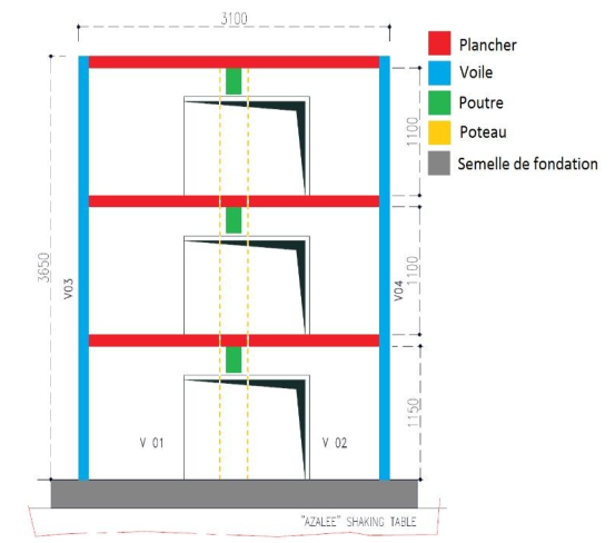
Figure 1.1-a : Dimensions of the Smart 2013 model (Elevation view — Dimensions in mm)
The thickness of the sails and slabs is 0.1 m. The thickness of the sole and the support of the pole is 0.25m.
The beams have a rectangular section \(0.325m\times 0.15m\).
The posts have a \(0.2m\times 0.2m\) square section.
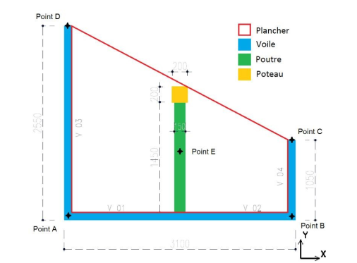
Figure 1.1-b : Dimensions of the Smart 2013 model (Plan view — Dimensions in mm)
1.2. Material properties#
The spring stiffness of the spring pad under the sole and the post support are:
k_x = 6.e8
k_y = 2.e8
k_z = 2.e9
k_rx=5.e9
k_ry = 5.e9
k_rz=1.e11
1.2.1. For load 1:#
Young’s module:.
Beams, posts, walls and slabs: \(E=14200\mathit{MPa}\)
Base and pole support: \(E=3200000\mathit{MPa}\)
Poisson’s ratio:.
Beams, posts and walls: \(\nu =0\)
Slabs, footing and pole support: \(\nu =\mathrm{0,2}\)
Density:
Beams, posts, sails, sole and pole support \(\rho =2500\mathit{kg}/m\mathrm{³}\)
Level 1 panel: \(\rho =2500+2450/0.1\mathit{kg}/m\mathrm{³}\)
Level 2 panel: \(\rho =2500+2570/0.1\mathit{kg}/m\mathrm{³}\)
Level 3 panel: \(\rho =2500+2150/0.1\mathit{kg}/m\mathrm{³}\)
Depreciation:
AMOR_ALPHA = 0.000454728
AMOR_BETA = 0.718078321
1.2.2. For load 2:#
Young’s module:.
Beams, posts and walls: \(E=32000\mathit{MPa}\)
Tiles: \(E=16000\mathit{MPa}\)
Base and pole support: \(E=3200000\mathit{MPa}\)
Poisson’s ratio:.
Beams, posts and walls: \(\nu =0\)
Slabs, footing and pole support: \(\nu =\mathrm{0,2}\)
Density:
Beams \(\rho =2500\mathit{kg}/m\mathrm{³}\)
Level 1 panel: \(\rho =2500+2450/0.1\mathit{kg}/m\mathrm{³}\)
Level 2 panel: \(\rho =2500+2570/0.1\mathit{kg}/m\mathrm{³}\)
Level 3 panel: \(\rho =2500+2150/0.1\mathit{kg}/m\mathrm{³}\)
Depreciation:
AMOR_ALPHA = 0.000454728
AMOR_BETA = 0.718078321
1.3. Boundary conditions and loads#
1.3.1. Loading 1#
The structure is subject to its own weight.
1.3.2. Loading 2#
The structure is subject to seismic stresses.
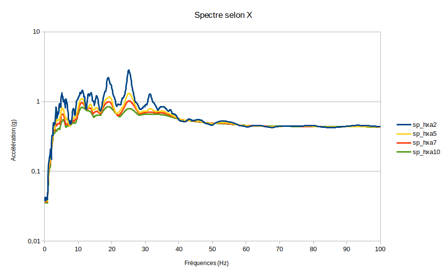
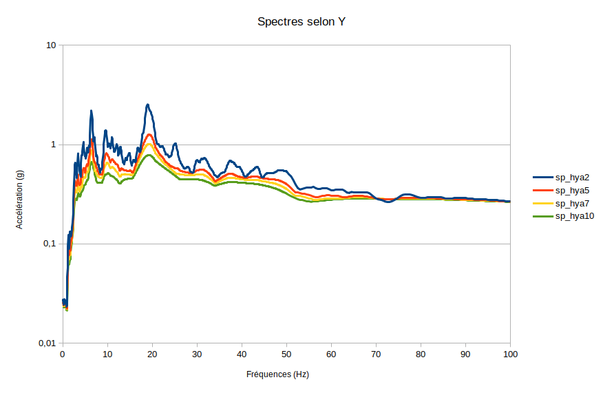
Combination CQC (Full Quadratic Combination) is calculated via COMB_SISM_MODAL for the spectra described below.
Next X:
Spectrum SP_HXa2 has a damping of 0.02.
Spectrum SP_HXa5 has a damping of 0.05.
Spectrum SP_HXa7 has a damping of 0.07.
Spectrum SP_HXa10 has a damping of 0.1.
Next Y:
Spectrum SP_HYa2 has a damping of 0.02.
Spectrum SP_HYa5 has a damping of 0.05.
Spectrum SP_HYa7 has a damping of 0.07.
Spectrum SP_HYa10 has a damping of 0.1.
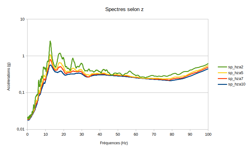
Next Z:
Spectrum SP_HZa2 has a damping of 0.02.
Spectrum SP_HZa5 has a damping of 0.05.
Spectrum SP_HZa7 has a damping of 0.07.
Spectrum SP_HZa10 has a damping of 0.1.
The combination CQCS is then deduced and used to evaluate the field resulting from the seismic calculation.