2. Modeling A#
2.1. Workflow of the TP#
2.1.1. Geometry and meshing with Salome-Meca#
Under Salomé-Méca, realize the geometry.
We can consider a plate centered at the origin, with a finite dimension: \(2m\) on the side.
Make the mesh. Remember that cracks are not meshed, so it is possible to use a regulated mesh of quadrangles that is sufficiently fine everywhere (1D algorithm = Wire discretization + 2D algorithm = Quadrangle).
2.1.2. Creating the command file without post-processing the break#
2.1.2.1. Reading the healthy mesh and defining the non-enriched model#
Reading the refined mesh (LIRE_MAILLAGE) in MED format; |
Definition of the finite elements used (AFFE_MODELE, MODELISATION =” D_PLAN “); |
Reorientation of the normals to the elements: we will use MODI_MAILLAGE/ORIE_PEAU_2Dpour to orient all the elements in the same way, with a normal turned towards the outside for the faces on which the load is applied; |
2.1.2.2. Definition of the crack and the elements X- FEM#
Definition of a single horizontal crack of length \(\mathrm{2a}\mathrm{=}\mathrm{0,3}m\) (DEFI_FISS_XFEM): preferably use the crack catalog (FORM_FISS =” SEGMENT “) |
Modifying the model to take into account the elements X- FEM (MODI_MODELE_XFEM), |
2.1.2.3. Definition of the material, the conditions and the resolution of the mechanical problem#
Material definition and assignment (DEFI_MATERIAU and AFFE_MATERIAU); |
Definition of limit conditions and loads (AFFE_CHAR_MECA) on the enriched model: * Blocking rigid modes (DDL_IMPOsur the GROUP_NO “N_A”, “N_B”); * Applying traction (1 MPa) on “M_up” and “M_down” (PRES_REP) |
Solving the elastic problem (MECA_STATIQUE) on the rich model. |
2.1.2.4. Post-processing of movements and constraints with X- FEM and visualization with Paravis#
Creating a visualization mesh (POST_MAIL_XFEM); |
Creating a model for visualization (AFFE_MODELE) on the mesh created for visualization; |
Creation of a results field on the X- FEM visualization mesh (POST_CHAM_XFEM); |
Print results in MED (IMPR_RESU) format. |
Complete the order file created by taking into account 2 cracks, in the following case:
\(a\mathrm{=}\mathrm{0,15}\) and \(b\mathrm{=}\mathrm{0,4}\) (i.e. \(2a\mathrm{/}b\mathrm{=}\mathrm{0,75}\))
\(e\mathrm{=}0\)
It is reminded that every call DEFI_FISS_XFEM produces a crack. For 2 cracks, you have to call this command twice.
2.1.3. Add break post-processing to the command file#
Calculating K with CALC_G
Calculate the stress intensity factor (K1) (OPTION =” CALC_K_G “).
Use the result of MECA_STATIQUE (RESULTAT).
Complete the information on field THETA:
the crack bottom, specifying the bottom number (in your case there are 2 crack bottoms A and B)
the radii of the crown of the theta field (R_INF, R_SUP), to be defined according to the mesh used.
The CALC_Gproduisant command has a table-like data structure, you have to print the results in a table with IMPR_TABLE.
Calculating K with POST_K1_K2_K3
Calculate K with POST_K1_K2_K3:
use the result of MECA_STATIQUE (RESULTAT)
fill in the bottom of the crack
fill in the ABSC_CURV_MAXI parameter
print the results in a table (IMPR_TABLE)
Note: do not take into account the alarm in CALC_CHAMP which states that EXCIT must be added.
Compare the results obtained to the Handbook solution.
To go further, we can:
extend the charts for \(2a\mathrm{/}r>0.9\) (for example \(2a\mathrm{/}r\mathrm{=}1\)),
study the fineness of the mesh,
do a parametric study for \(e\mathrm{=}\mathrm{[}\mathrm{0 };\mathrm{2b}\mathrm{]}\) (think about using python),
study other configurations (inclined cracks, addition of other cracks…).
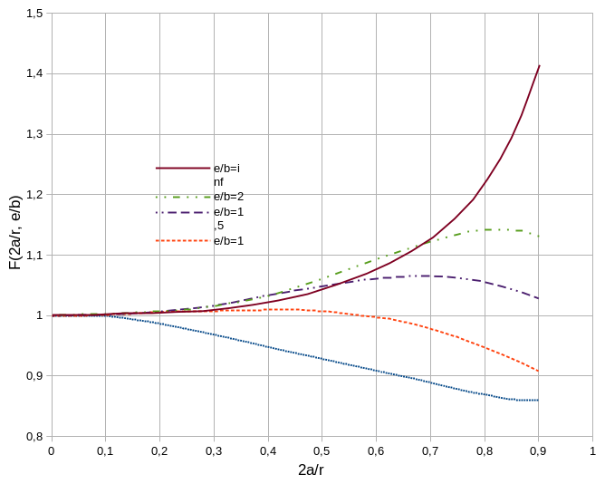
Figure 2.1.3-1: Abacus