3. Modeling A#
3.1. Characteristics of modeling A#
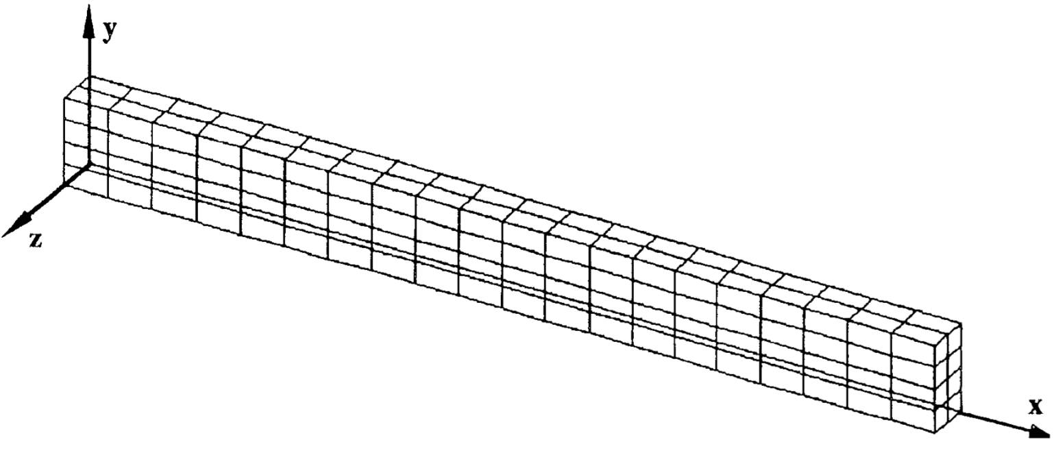
Figure 3.1-1: Problem geometry mesh
In this modeling, the complete structure is meshed using 3D solid elements.
The flatness constraint is expressed as follows. Be it,
point A \(X=0\), \(Y=h/2\), \(Z=0\): \(\mathit{DX}=\mathit{DY}=0\), \(\mathit{DZ}\ne 0\);
point B \(X=0\), \(Y=h/2\), \(Z=b\): \(\mathit{DX}=\mathit{DY}=0\), \(\mathit{DZ}\ne 0\);
the C point \(X=0\), \(Y=h\), \(Z=b/2\): \(\mathit{DX}\ne \mathit{DY}\ne 0\), \(\mathit{DZ}=0\)
By neglecting second-order terms in displacements, the flatness constraint results in a linear relationship between the \(\mathit{DX}=0\) displacements of the points \(A\), \(B\), \(C\) and \(P\), any point on the face:
\(∣\begin{array}{cccc}{\mathit{DX}}_{P}& {Y}_{P}& {Z}_{P}& 1\\ {\mathit{DX}}_{A}& h/2& 0& 1\\ {\mathit{DX}}_{B}& h/2& b& 1\\ {\mathit{DX}}_{C}& h& b/2& 1\end{array}∣=0\)
The condition is then written for \({\mathit{DX}}_{A}=0\):
\({\mathit{DX}}_{P}={\mathit{DX}}_{C}\times (\frac{2{Y}_{P}}{h-1})\)
In \(X=L\), the flatness condition is obtained in the same way but for any \({\mathit{DX}}_{A}\). The relationship is then written:
\({\mathit{DX}}_{P}={\mathit{DX}}_{C}\times (\frac{2{Y}_{P}}{h-1})+2\times (1-\frac{{Y}_{P}}{h})\times {\mathit{DX}}_{A}\)
3.2. Characteristics of the mesh#
Number of knots: 1077
Number of meshes and types: 160 HEXA20
3.3. Tested sizes and results#
Mode |
Reference Value |
Reference Type |
Tolerance (%) |
1 |
|
“ANALYTIQUE” |
\(1.0\) |
2 |
|
“ANALYTIQUE” |
\(1.0\) |
3 |
|
“ANALYTIQUE” |
\(1.0\) |
4 |
|
“ANALYTIQUE” |
\(1.0\) |
5 |
|
“ANALYTIQUE” |
\(1.0\) |