4. B modeling#
4.1. Characteristics of modeling#
It is a system of shafts rotating along the \(Z\) axis with negative rotation speeds. To obtain the same results as modeling A (with the minus sign), you must put a minus sign on the cross terms of the stiffness and damping matrices. The characteristics of the bearings are indicated in the following table.
Level |
\(\mathrm{P1}\) |
|
|
\({K}_{\mathit{yx}}\mathrm{=}{1.10}^{7}N\mathrm{/}m\) |
|
||
\({C}_{\mathrm{yy}}=8.{10}^{3}\mathrm{Ns}/m\) |
|
||
\({C}_{\mathit{yx}}\mathrm{=}3.{10}^{3}\mathit{Ns}\mathrm{/}m\) |
|
||
Level |
\(\mathrm{P2}\) |
|
|
\({K}_{\mathit{yx}}\mathrm{=}2.{10}^{6}N\mathrm{/}m\) |
|
||
\({C}_{\mathrm{yy}}=6.{10}^{3}\mathrm{Ns}/m\) |
|
||
\({C}_{\mathit{yx}}\mathrm{=}1.5{10}^{3}\mathit{Ns}\mathrm{/}m\) |
|
Therefore, the precessions of the modes are also reversed, that is, the direct modes become retrograde and vice versa.
4.2. Characteristics of the mesh#
The rotor is meshed in 12 finite shaft elements of type POU_D_T and includes 4 discrete elements of type DIS_TR for modeling disks and bearings.
Number of knots: 13
Number and type of elements: 12 SEG2
4 POI1
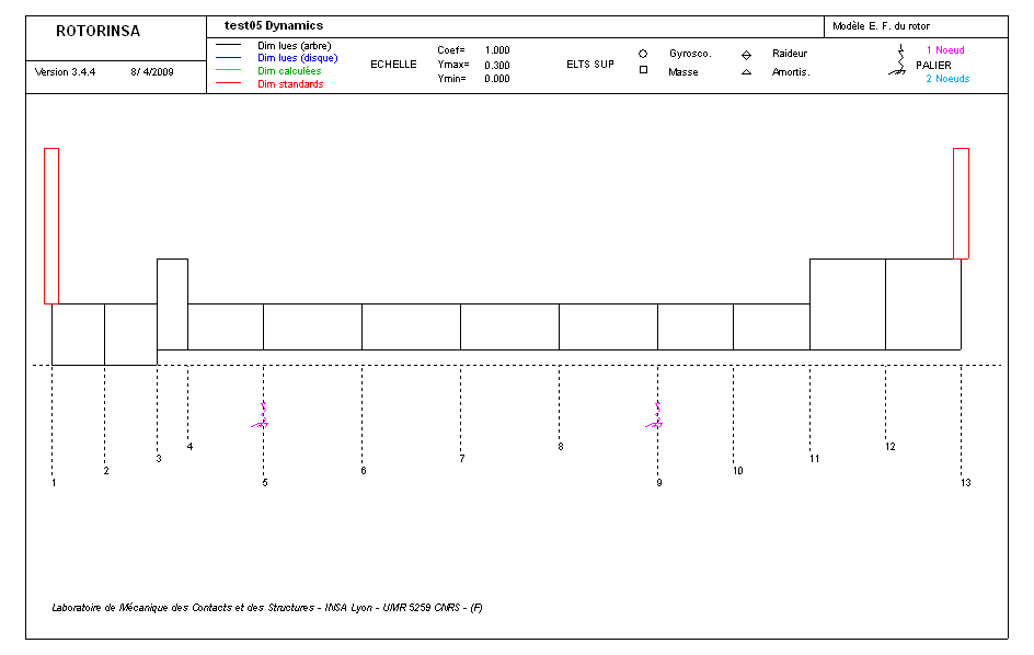
Figure 1-b: Characteristic of the finite element model under ROTORINSA
4.3. Tested sizes and results#
4.3.1. Natural frequencies as a function of rotation speed#
The values of the first 8 bending frequencies for speeds \(0\mathrm{tr}/\mathrm{mn}\) and \(-60000\mathrm{tr}/\mathrm{mn}\), for both software programs, are shown in the table below.
Freq number in flexion |
Rotation speed ( \(\mathrm{tr}/\mathrm{min}\) ) |
ROTORINSA |
Aster_code |
||
\(∣F∣(\mathrm{Hz})\) |
Damping factor |
Tolerances of \(∣F∣(\mathrm{Hz})\) |
Damping tolerances reduced |
||
A1 |
0 |
2.16212E+02 |
4.76544E-02 |
1.E-3 |
1.E-3 |
-60000 |
1.85365E+02 |
-5.17463E-02 |
1.E-3 |
1.1E-3 |
|
2 |
0 |
2.63539E+02 |
7.87281E-02 |
1.E-3 |
6.E-3 |
-60000 |
2.96078E+02 |
1.55245E-01 |
1.E-3 |
5.E-3 |
|
3 |
0 |
3.83210E+02 |
5.01438E-02 |
1.E-3 |
14.E-3 |
-60000 |
3.24718E+02 |
1.57489E-03 |
1.E-3 |
70.E-3 |
|
4 |
0 |
4.39642E+02 |
6.02275E-02 |
1.E-3 |
12.E-3 |
-60000 |
4.72541E+02 |
1.59683E-01 |
1.2E-3 |
3.E-3 |
|
Table 2-a: Flexion-type natural frequencies for Code_Aster and ROTORINSA
The frequencies obtained are in perfect harmony with those of ROTORINSA.
There is an instability of the first mode, which appears at \(-16760\mathrm{tr}/\mathrm{mn}\).
In Code_Aster, we also observe frequencies and modes of torsion and modes of traction/compression. These modes are not calculated by ROTORINSA, as it only models bending behavior. The values of these frequencies are tested in NON_REGRESSION and only when stopped. In fact, the modes of twisting and pulling are, by definition, invariant with respect to the speed of rotation.