3. Modeling A#
3.1. Characteristics of modeling#
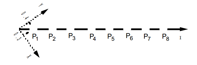
Discrete translational stiffness element DIS_T
Characteristics of the elements:
ORIENTATION: |
in all the nodes |
with an angle \(\alpha \mathrm{=}53.130102°\) |
DISCRET: |
|||
with nodal masses all nodes |
M_T_D_N |
in absolute coordinate system |
\((m\mathrm{=}10.)\) |
all-mesh stiffness matrices |
K_T_D_L |
in local coordinate system |
\((\mathit{Kx}\mathrm{=}1.{10}^{5})\) |
at the end nodes |
K_T_D_N |
in local coordinate system |
\(({K}_{x}\mathrm{=}1.{10}^{5})\) |
Boundary conditions:
DDL_IMPO: (TOUT: “OUI” DZ: 0.)
LIAISON_DDL: (such as \(\mathrm{3Dy}\mathrm{=}\mathrm{4Dx}\) in all nodes)
Node names: \({P}_{\mathrm{1,}}{P}_{\mathrm{2,}}\mathrm{....},{P}_{8}\)
: label: EQ-None
mathit {Point} Amathrm {=}mathit {N1}
3.2. Characteristics of the mesh#
Number of knots: 8
Number of meshes and types: 7 SEG2
3.3. Tested sizes and results#
Identification Clean mode number |
Reference |
1 |
5.5274 |
2 |
10.8868 |
3 |
15.9155 |
4 |
20.4606 |
5 |
24.3840 |
6 |
27.5664 |
7 |
29.9113 |
8 |
31.3474 |
Standardized mode with 1 to the largest component
Nature of clean modes |
Point |
Reference |
Translation 1 (\(\mathit{Dy}\)) \({\Phi }_{1}\) |
P1 P2 P3 P4 P5 P6 P7 P8 |
—0.3473 —0.6527 —0.8793 —1. —1. —0.8793 —0.6527 —0.3473 |
Translation 8 (\(\mathit{Dy}\)) \({\Phi }_{8}\) |
P1 P2 P3 P4 P5 P6 P7 P8 |
0.3473 —0.6527 0.8793 —1. 1. —0.8793 0.6527 —0.3473 |
Maximum error less than: 0.03%.
Mode standardized to the generalized unit mass
Nature of clean modes |
Point |
Reference |
Translation 1 (\(\mathit{Dy}\)) \({\Phi }_{1}\) |
P1 P2 P3 P4 P5 P6 P7 P8 |
—4.0781E—2 —7.6654E—2 —1.0327E—1 —1.1743E—1 —1.1743E—1 —1.0327E—1 —7.6654E—2 —4.0781E—2 |
Translation 8 (\(\mathit{Dy}\)) \({\Phi }_{8}\) |
P1 P2 P3 P4 P5 P6 P7 P8 |
4.0781E—2 —7.6654E—2 1.0327E—1 —1.1743E—1 1.1743E—1 —1.0327E—1 7.6654E—2 —4.0781E—2 |
Maximum error less than: 0.03%.
Standardized mode with unitary generalized stiffness
Nature of clean modes |
Point |
Reference |
Translation 1 (\(\mathit{Dy}\)) \({\Phi }_{1}\) |
P1 P2 P3 P4 P5 P6 P7 P8 |
—1.1742E—3 —2.2072E—3 —2.9735E—3 —3.3813E—3 —3.3813E—3 —2.9735E—3 —2.2072E—3 —1.1742E—3 |
Translation 8 (\(\mathit{Dy}\)) \({\Phi }_{8}\) |
P1 P2 P3 P4 P5 P6 P7 P8 |
2.0705E—4 —3.8918E—4 5.2432E—4 —5.9621E—4 5.9621E—4 —5.2432E—4 3.8918E—4 —2.0705E—4 |
Maximum error less than: 0.03%.
We are also testing the INFO_MODE command. Since GEP is standard (real symmetric matrices) its eigenvalues belong only to the real axis. In this case, we can therefore compare the two counting methods (COMPTAGE/METHODE =” STURM “and” APM “) and check that they actually give the same results.
We thus determine the number of eigenvalues (NB_FREQ) contained strictly in a frequency band [FREQ_MIN, FREQ_MAX] (if Sturm) or in the disk with center FREQ_CENTRE and radius, in frequency, \(\frac{\sqrt{\text{FREQ\_RAYON\_CONTOUR}}}{2\pi }\) (if APM). We specify the counting method used (Sturm or APM).
Concept |
FREQ_MIN/ FREQ_CENTRE |
FREQ_RAYON_ CONTOUR |
|
Counting method |
|
NBMOD01 |
0.0 |
5 |
5 |
0 |
Sturm |
NBMOD02 |
0.0 |
21 |
4 We count \({({\lambda }_{i})}_{\text{i=1,4}}\) |
Sturm |
|
NBMOD03 |
0.0 |
32 |
8 We count \({({\lambda }_{i})}_{\text{i=1,8}}\) |
Sturm |
|
NBMOD11 |
0.0+0.0j |
986.96 (= \({(5\mathrm{\times }2\pi )}^{2}\)) |
0 Same NBMOD01 |
|
|
NBMOD12 |
0.0+0.0j |
1740.99 (= \({(21\mathrm{\times }2\pi )}^{2}\)) |
4 Same NBMOD02 |
|
|
NBMOD13 |
0.0+0.0j |
4042.58 |
|||
(= \({(32\mathrm{\times }2\pi )}^{2}\)) » |
8 Same NBMOD03 |
|
|||
NBMOD4 |
(= \({(\mathrm{15.91x2}\pi )}^{2}\)) |
5000.0 |
1 We count \({\lambda }_{1}\) |
|
|
NBMOD5 |
|
900.0 |
0 |
|
3.4. notes#
Calculations made by:
CALC_MODES

OPTION =' AJUSTE ',
CALC_FREQ =_F (FREQ =( 5., 10., 10., 15., 15., 15., 15., 15., 20., 24., 24., 27., 30., 32.)), SOLVEUR_MODAL =_F (OPTION_INV =” DIRECT “)
Contents of the results file:
8 first natural frequencies, eigenvectors and modal parameters