1. Reference problem#
1.1. Geometry#
It is a material point, representative of a state of homogeneous stresses and deformations.
1.2. Material properties#
1.2.1. Umat data#
The coefficients of Umat behavior are (cf. [U4.43.01]):
\(\mathrm{C1}=\lambda =\frac{E\nu }{(1+\nu )(1-2\nu )}\)
\(\mathrm{C2}=\mu =\frac{E}{2(1+\nu )}\)
\(\mathrm{C3}=\tilde{\lambda }=\frac{\lambda }{20}\)
\(\mathrm{C4}=\tilde{\mu }=\frac{\mu }{20}\)
\(\mathrm{C5}=\tilde{\nu }=0\)
We will use: DEFI_MATERIAU/UMAT =_F (LISTE_COEF =( C1, C2, C3, C4, C5)),
1.3. Boundary conditions and loads#
The load is the same as in tests COMP001, see [V6.07.101].
1.3.1. Characteristics of loading paths#
The proposed loading causes each component of the deformation tensor to vary in a decoupled manner by successive step. A cyclic load-discharge path is proposed by covering the states of traction and compression as well as an inversion of the signs of shear in order to test a wide range of values.
Schematically, it follows a course on 8 segments \([O-A-B-C-O-C’-B’-A’-O]\) where the second part of the path \([O-C’-B’-A’-O]\) is symmetric with respect to the origin of the first \([O-A-B-C-O]\).
1.3.2. Application of requests#
We come back to the study of a material point (using the macro-command SIMU_POINT_MAT [U4.51.12]) by stressing an element in a homogeneous manner by imposing in \(\mathrm{3D}\), the 6 components of the deformation tensor:
\(\stackrel{ˉ}{\varepsilon }=\left[\begin{array}{ccc}{\varepsilon }_{\mathrm{xx}}& {\varepsilon }_{\mathrm{xy}}& {\varepsilon }_{\mathrm{xz}}\\ {\varepsilon }_{\mathrm{xy}}& {\varepsilon }_{\mathrm{yy}}& {\varepsilon }_{\mathrm{yz}}\\ {\varepsilon }_{\mathrm{xz}}& {\varepsilon }_{\mathrm{yz}}& {\varepsilon }_{\mathrm{zz}}\end{array}\right]\)
For a more general description, the imposed deformation tensor will be decomposed into a hydrostatic and deviatoric part on shear bases:
\(\stackrel{ˉ}{\varepsilon }=\left[\begin{array}{ccc}{\varepsilon }_{\mathrm{xx}}& {\varepsilon }_{\mathrm{xy}}& {\varepsilon }_{\mathrm{xz}}\\ {\varepsilon }_{\mathrm{xy}}& {\varepsilon }_{\mathrm{yy}}& {\varepsilon }_{\mathrm{yz}}\\ {\varepsilon }_{\mathrm{xz}}& {\varepsilon }_{\mathrm{yz}}& {\varepsilon }_{\mathrm{zz}}\end{array}\right]=p\left[\begin{array}{ccc}1& 0& 0\\ 0& 1& 0\\ 0& 0& 1\end{array}\right]+{d}_{1}\left[\begin{array}{ccc}1& 0& 0\\ 0& -1& 0\\ 0& 0& 0\end{array}\right]+{d}_{2}\left[\begin{array}{ccc}0& 0& 0\\ 0& 1& 0\\ 0& 0& -1\end{array}\right]+\left[\begin{array}{ccc}0& {\varepsilon }_{\mathrm{xy}}& {\varepsilon }_{\mathrm{xz}}\\ {\varepsilon }_{\mathrm{xy}}& 0& {\varepsilon }_{\mathrm{yz}}\\ {\varepsilon }_{\mathrm{xz}}& {\varepsilon }_{\mathrm{yz}}& 0\end{array}\right]\) in 3D.
1.3.3. Description of the imposed deformation path in 3D#
The path applied is described in the table below, the deformation values applied are calibrated with respect to the elastic modulus:
Segment number |
1 |
2 |
2 |
3 |
3 |
3 |
4 |
5 |
6 |
7 |
8 |
Segment |
\(0-A\) |
|
|
|
|
|
|
|
|||
\({\varepsilon }_{\mathrm{xx}}\ast E\) |
787.5 |
1050 |
1050 |
350 |
350 |
0 |
-350 |
-1050 |
-787.5 |
0 |
|
\({\varepsilon }_{\mathrm{yy}}\ast E\) |
525.0 |
-175 |
-175 |
-350 |
-350 |
175 |
525 |
0 |
|||
\({\varepsilon }_{\mathrm{zz}}\ast E\) |
262.5 |
700 |
700 |
-525 |
-525 |
525 |
-700 |
-262.5 |
0 |
||
\({\varepsilon }_{\mathrm{xy}}\ast E/(1+\nu )\) |
700 |
350 |
350 |
1050 |
1050 |
-1050 |
-350 |
-700 |
0 |
||
\({\varepsilon }_{\mathrm{xz}}\ast E/(1+\nu )\) |
-350 |
350 |
350 |
700 |
700 |
0 |
-700 |
700 |
0 |
||
\({\varepsilon }_{\mathrm{yz}}\ast E/(1+\nu )\) |
0 |
700 |
-350 |
-350 |
0 |
350 |
-700 |
0 |
0 |
||
\(P\) |
525 |
525 |
525 |
-175 |
-175 |
-525 |
-525 |
0 |
|||
\(\mathrm{d1}\) |
262.5 |
525 |
525 |
525 |
0 |
-525 |
-525 |
-262.5 |
0 |
||
\(\mathrm{d2}\) |
262.5 |
-175 |
-175 |
350 |
350 |
0 |
-350 |
175 |
-262.5 |
0 |
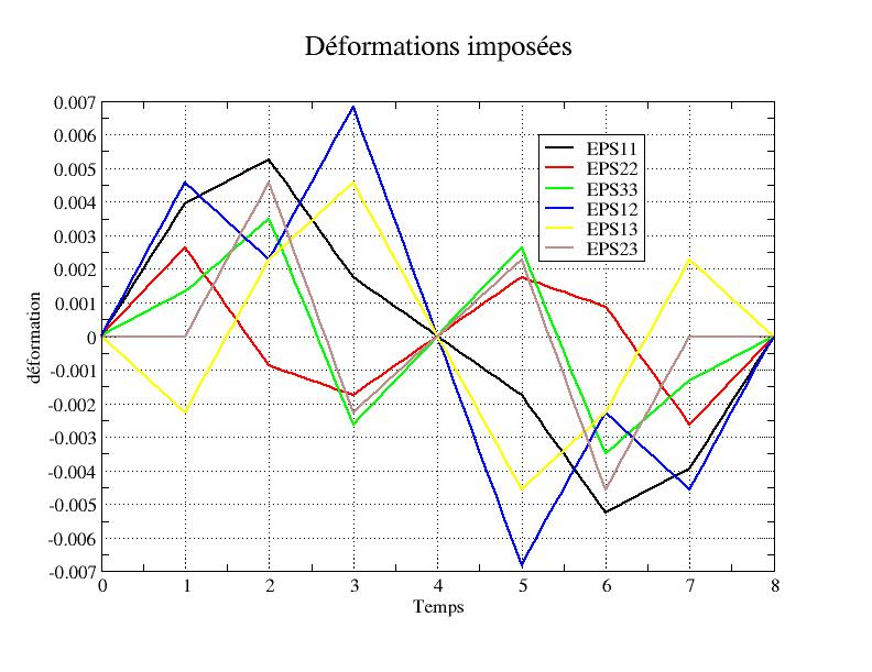
This path is illustrated by the following graph:
1.4. Initial conditions#
Zero stresses and deformations.