3. Modeling A#
3.1. Characteristics of modeling#
3D modeling is used.
3.2. Characteristics of the mesh#
The 3D mesh contains 100 elements of type HEXA8 of dimension \(0.4\mathrm{\times }0.4\mathrm{\times }0.2\mathit{mm}\):
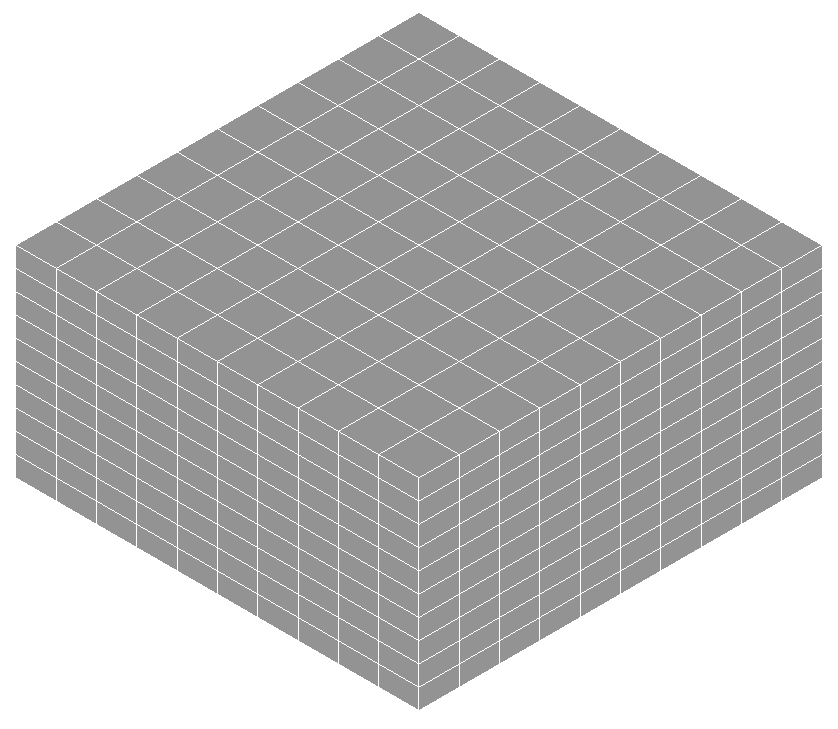
Figure 3.2-1: mesh used
For the auxiliary grid, a 3D mesh containing 400 elements of type HEXA8 of dimension \(0.2\mathrm{\times }0.2\mathrm{\times }0.1\mathit{mm}\) is used:
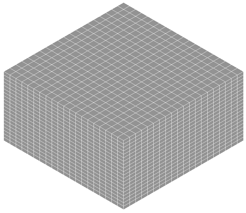
Figure 3.2-2: Auxiliary grid
3.3. Tested sizes and results#
After the two imposed propagations, we calculate the values of the level sets at the points of intersection between the segment connecting the end points of the background \((\mathrm{0,2}.189\mathrm{,0}.156)\) and \((\mathrm{4,2}.189\mathrm{,0}.156)\) (see § 2.2) and the faces of the elements of the mesh and we will check that the maximum and minimum values obtained are equal to zero. Assuming that the mesh is coarse, a tolerance equal to 15% of the length of the smallest edge of the mesh is used, i.e. \(0.15\mathrm{\cdot }0.2\mathit{mm}\mathrm{=}0.03\mathit{mm}\). So we accept the value of the level set at the bottom point in question if and only if it is in the interval \(\mathrm{[}\mathrm{-}0.03\mathrm{,0}.03\mathrm{]}\).