1. Modeling A#
1.1. Characteristics of modeling#
This test case proposes a number of analytical tests of the random signal generation operator GENE_FONC_ALEA. This operator generates realizations of a stationary Gaussian random process characterized by its power spectral density (DSP). We consider a two-dimensional DSP with \({S}_{1}\) and \({S}_{2}\) auto-spectra shown in Figure 1 below.
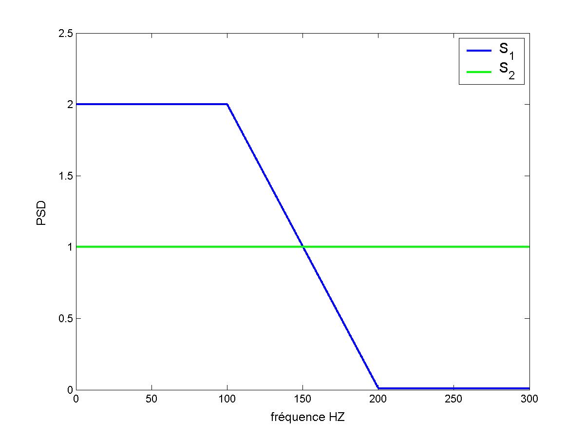
Figure 1: Auto-spectrum look \({S}_{1}\) and \({S}_{2}\)
The interspectrum is written as \({S}_{12}(f)\mathrm{=}\rho {({S}_{1}(f){S}_{2}(f))}^{\mathrm{0,5}}{e}^{i2\pi fT}\) where \(T\mathrm{=}\mathrm{0,025}\) and \({\rho }^{2}\mathrm{=}\mathrm{0,8}\) is the correlation coefficient. The standard deviations are \({\sigma }_{1}\mathrm{=}\sqrt{(603.)}\) and \({\sigma }_{2}=\sqrt{(600.)}\) respectively.
We are also testing the construction of DSP via POST_DYNA_ALEA, the operator for statistical post-processing of DSP.
Random signals are drawn by operator GENE_FONC_ALEA
DSP are estimated with the CALC_INTE_SPEC operator
We perform statistical post-processing of DSP with the POST_DYNA_ALEA operator
INFO_FONCTION is used to estimate the standard deviation of a given signal
1.2. Tested sizes and results#
1.2.1. Signal generation with interpolation and imposed duration#
Identification |
Reference |
% Tolerance |
Type |
|
Autospectrum standard deviation \({S}_{1}\) |
|
1.0 10—5 |
Analytics |
|
Autospectrum standard deviation \({S}_{2}\) |
|
1.0 10—5 |
Analytics |
|
Signal standard deviation 1 |
|
1.0 10—3 |
analytical |
|
Signal standard deviation 2 |
|
1.0 10—3 |
analytical |
|
Autospectrum standard deviation signal 1 |
|
1.0 10—3 |
analytical |
Autospectrum standard deviation signal 2 |
|
1.0 10—3 |
analytical |
|
Moment order 0 autospectrum signal 1 |
|
1.0 10—2 |
analytical |
|
Moment order 0 autospectrum signal 1 |
|
1.0 10—2 |
analytical |
|
Moment order 1 autospectrum signal 1 |
|
1.0 10—3 |
Non-regression |
|
Moment order 1 autospectrum signal 1 |
|
1.0 10—2 |
analytical |
We also test (with respect to analytical values and in non-regression) the RMS values of the estimated autospectra.
1.2.2. Signal generation with interpolation, imposed number of points#
Identification |
Reference |
Tolerance |
Type |
Signal standard deviation 1 |
|
|
Analytics |
Signal standard deviation 2 |
|
|
Analytics |
1.2.3. Signal generation with interpolation, nothing imposed, truncation of 10-100Hz#
Identification |
Reference |
Tolerance |
Type |
Signal standard deviation 1 |
|
|
Analytics |
Signal standard deviation 2 |
|
|
Analytics |
1.2.4. Signal generation with interpolation, number of points and imposed duration#
Identification |
Reference |
Tolerance |
Type |
Signal standard deviation 1 |
|
|
Analytics |
Signal standard deviation 2 |
|
|
Analytics |
1.2.5. Signal generation with interpolation#
Identification |
Reference |
Tolerance |
Type |
Signal standard deviation 1 |
|
|
Analytics |
Signal standard deviation 2 |
|
|
Analytics |
1.2.6. Generating signals without interpolation#
Identification |
Reference |
Tolerance |
Type |
Signal standard deviation 1 |
|
|
Analytics |
Signal standard deviation 2 |
|
|
Analytics |
1.2.7. Signal generation without interpolation, imposed number of points#
Identification |
Reference |
Tolerance |
Type |
Signal standard deviation 1 |
|
|
Analytics |
Signal standard deviation 2 |
|
|
Analytics |