1. Reference problem#
1.1. Modeling A#
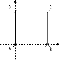
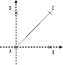
1.1.1. Geometry#

|
|
|
\(\mathrm{Carre1}/\mathrm{carre2}\) \(\mathrm{AC}\) \(\mathrm{cube1}\)
Coordinates of points \((m)\):
\(A:(0.,0.)\)
\(B:(1.,0.)\)
\(C:(0.,0.)\)
\(D:(0.,1.)\)
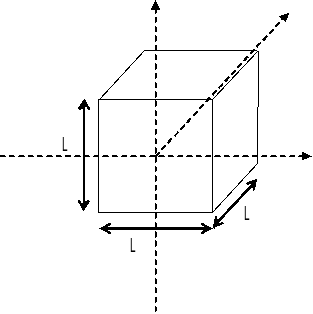
Cube geometry:
Center: \((0.,0.,-0.5)\)
Side: \(L=1\)
Mesh group:
\(\mathrm{carre}1\) surface \(A,B,C,D\)
\(\mathrm{carre}2\) surface \(A,B,C,D\)
\(\mathrm{AC}\) segment \(\mathrm{AC}\)
\(\mathrm{cube1}\) volume
1.1.2. Material properties#
Not applicable
1.1.3. Boundary conditions and loads#
Not applicable
1.2. Benchmark solution#
1.2.1. Calculation method#
Calculating the reference for the temperature field
The field that is projected from one model to the other is an analytical temperature field whose evolution is as follows:
\(T=3.+X+Y\)
The reference solution is identical to the projected analytical field.
Calculating the reference for the constraint field
The objective is to change the coordinate system, after projecting a known stress field onto a mesh into a 3D mesh.
Transition from a cylindrical coordinate system (\(\mathrm{XOY}\)) to a Cartesian coordinate system \(\mathrm{3D}\) (\(\mathrm{XYZ}\)).
The constraint field \((N/{m}^{2})\) in the axisymmetric coordinate system (axis \(\mathrm{OY}\)) is as follows:
\(\mathrm{SIXX}=2\)
\(\mathrm{SIYY}=y\)
\(\mathrm{SIZZ}=1\)
\(\mathrm{SIXY}=0.\)
The constraint field in the Cartesian coordinate system (\(\mathrm{3D}\)) is obtained by performing:
A projection of the stress tensor evaluated on mesh \(\mathrm{2D}\mathrm{axis}\) onto the 3D mesh.
Change of frame of the stress tensor \([{\sigma }_{\mathrm{3D}}]=[P][{\sigma }_{\mathrm{cyl}}]{[P]}^{T}\) or \([P]\) represents the change of frame matrix.
The numerical results are as follows:
NOEUD |
|
|
|
|
|
|
|||||||
N258 |
-1/3 |
-1/3 |
-1/3 |
1/3 |
1/3 |
1/3 |
1/3 |
1/3 |
1/3 |
1/3 |
1/3 |
1/3 |
1/6 |
N33 |
-1/3 |
||||||||||||
N108 |
1/2 |
2/3 |
2/3. |
1.2.2. Benchmark results#
Projection type |
Point |
Size \((°C)\) |
Reference |
\(\mathrm{carre1}\to \mathrm{carre2}\) |
\(A\) |
\(\mathrm{TEMP}\) |
\(3\) |
\(B\) |
\(\mathrm{TEMP}\) |
\(4\) |
|
\(C\) |
\(\mathrm{TEMP}\) |
\(5\) |
|
\(\mathrm{N364}\) |
\(\mathrm{TEMP}\) |
\(4.66\) |
|
\(\mathrm{carre2}\to \mathrm{carre1}\) |
\(A\) |
\(\mathrm{TEMP}\) |
\(3\) |
\(B\) |
\(\mathrm{TEMP}\) |
\(4\) |
|
\(C\) |
\(\mathrm{TEMP}\) |
\(5\) |
|
\(\mathrm{N355}\) |
\(\mathrm{TEMP}\) |
\(3.75\) |
|
\(\mathrm{carre2}\to \mathrm{AC}\) |
\(A\) |
\(\mathrm{TEMP}\) |
\(3\) |
\(C\) |
\(\mathrm{TEMP}\) |
\(5\) |
|
\(\mathrm{N356}\) |
\(\mathrm{TEMP}\) |
\(4\) |
|
\(\mathrm{AC}\to \mathrm{carre2}\) |
\(A\) |
\(\mathrm{TEMP}\) |
\(3\) |
\(B\) |
\(\mathrm{TEMP}\) |
\(4\) |
|
\(\mathrm{carre2}\to \mathrm{cube1}\) |
\(C\) |
\(\mathrm{TEMP}\) |
\(5\) |
\(\mathrm{N363}\) |
\(\mathrm{TEMP}\) |
\(3.33\) |
|
\(\mathrm{N341}\) |
\(\mathrm{TEMP}\) |
\(3.69371\) |
Projection type |
Point |
Size \((N/{m}^{2})\) |
Reference |
\(\mathrm{carre2}\to \mathrm{cube1}\) |
\(\mathrm{N258}\) |
\(\mathrm{SIXX}\) |
\(1.5\) |
\(\mathrm{N258}\) |
\(\mathrm{SIYY}\) |
\(1.5\) |
|
\(\mathrm{N258}\) |
\(\mathrm{SIZZ}\) |
\(0.16\) |
|
\(\mathrm{N33}\) |
\(\mathrm{SIXX}\) |
\(2\) |
|
\(\mathrm{N33}\) |
\(\mathrm{SIYY}\) |
\(1\) |
|
\(\mathrm{N33}\) |
\(\mathrm{SIZZ}\) |
\(1\) |
|
\(\mathrm{N108}\) |
\(\mathrm{SIXX}\) |
\(1\) |
|
\(\mathrm{N108}\) |
\(\mathrm{SIYY}\) |
\(2\) |
|
\(\mathrm{N108}\) |
\(\mathrm{SIZZ}\) |
\(0.66\) |
1.3. B modeling#
1.3.1. Geometry#

Cube side: \(L=2\)
1.3.2. Material properties#
\(E=2N/{m}^{2}\)
\(\nu =0.\)
1.3.3. Boundary conditions and loads#
Compulsory trips
plan \(z=\mathrm{1m}\) \(\mathrm{DX}=0.=\mathrm{DY}=0.=\mathrm{DZ}=0.\)
plan \(z=3m\) \(\mathrm{DZ}=\mathrm{2.m}\)
1.4. Benchmark solution#
1.4.1. Calculation method#
The Poisson ratio is zero \(\nu =0\) which gives us
\({\sigma }_{\mathrm{xx}}={\sigma }_{\mathrm{yy}}={\sigma }_{\mathrm{xy}}={\sigma }_{\mathrm{xz}}={\sigma }_{\mathrm{yz}}=0\)
\({\sigma }_{\mathrm{zz}}=E\epsilon =E\frac{\mathrm{DZ}}{L}\)
1.4.2. Benchmark results#
\(\mathrm{SIZZ}=2N/{m}^{2}\) At any point in the cube