3. C modeling#
3.1. Characteristics of modeling#
25 POU_D_T beam elements,
5 node-node connection elements (DIS_TR_L),
26 point mass POI1 elements (DIS_TR_N),
2 elements POI1 with zero point mass (DIS_T) to model control points in the soil to be post-treated,
136 solid elements (“3D” modeling) for the base and 136 DST elements for its underside.
1st harmonic calculation: in the interval \((\mathrm{0,10}\mathit{Hz})\) in steps of \(0.1\mathit{Hz}\),
2nd harmonic calculation: in the interval \((\mathrm{0,10}\mathit{Hz})\) in steps of \(0.1\mathit{Hz}\),
3rd transitional calculation: in the interval \((\mathrm{0,10}s)\) in steps of \({10}^{\mathrm{-}2}s\).
This modeling is characterized by the presence of control points in the ground in order to model the deconvolution of a vertical sinusoidal signal imposed on the ground surface.
3 elements POI1 with zero point mass (DIS_T) are thus introduced in order to model control points in the soil to be post-treated.
They correspond to 3 levels at the depth of a homogeneous ground: on the surface and offset respectively by a quarter and a half plane pressure wave length at vertical incidence.
This soil is a homogeneous soil whose characteristics are summarized in the table below:
Layer |
Thickness ( \(m\) ) |
\(\rho\) ( \(\mathit{kg}\mathrm{/}{m}^{3}\) ) |
\(\nu\) |
( \(\mathit{MPa}\) ) |
||
Layer 1 |
35 |
2400 |
2400 |
0.4 |
70 |
0.1 |
Table 6.1-1: Mechanical characteristics of homogeneous soil
These values induce a pressure wave speed \({V}_{P}\mathrm{=}250m\mathrm{/}s\), which gives a pressure wave length of 50 meters for an excitation frequency of \(5\mathit{Hz}\). The second and the third control points are therefore pressed by \(12.5m\) and \(25m\) respectively in the vertical direction.
A transient calculation is carried out in the interval \((\mathrm{0,4}s)\) in steps of \({10}^{\mathrm{-}2}s\) with a sinusoidal acceleration of frequency \(5\mathit{Hz}\) imposed on the ground surface in the vertical direction \(Z\).
3.2. Characteristics of the mesh#
Number of knots: 190
Number of meshes and type: 136 PENTA6, 136 TRIA3, 136, 30 SEG2, 28 POI1
3.3. Reference solution#
For a sinusoidal load of frequency \(f\) in a ground with wave speed \(C\) and hysteretic damping \(\beta\), analytically, as an amplitude factor at depth \(Z\), we obtain:
\(\mathit{Az}=\mathit{sh}(\mathrm{\beta }\mathrm{\pi }fZ/C)\mathrm{sin}(2\mathrm{\pi }fZ/C)+\mathit{ch}(\mathrm{\beta }\mathrm{\pi }fZ/C)\mathrm{sin}(2\mathrm{\pi }fZ/C)\)
The corresponding amplitude in speed will then be:
\(\mathit{Vz}=\mathit{Az}/(2\mathrm{\pi }f)\)
And the corresponding amplitude in movement will therefore be:
\(\mathit{Dz}=-\mathit{Az}/{(2\mathrm{\pi }f)}^{2}\)
It can only be seen, by way of comparison, that the peaks of the harmonic responses correspond well to the resonance frequencies obtained with an equivalent ground spring model.
On the other hand, for the resolution in the frequency domain of the harmonic problem projected on a modal basis consisting of natural modes with a blocked interface and constrained static modes, the same results are obtained by Code_Aster and by MISS3D.
3.4. Tested sizes and results#
Transient calculation (real), resolution by MISS3D and post-processing at control points.
Calculation with accelerogram provided on a time basis:
Calculation with accelerogram provided on a frequency basis:
The reference is provided by the calculation with an accelerogram on a time basis.
Identification |
Reference Value |
Reference Type |
Tolerance |
|
Transfer, \(\mathit{FREQ}=5\), Point \(\mathit{NC1}\) |
9.95035E-01 - 9.95046E-02j |
“AUTRE_ASTER” |
0, 1% |
|
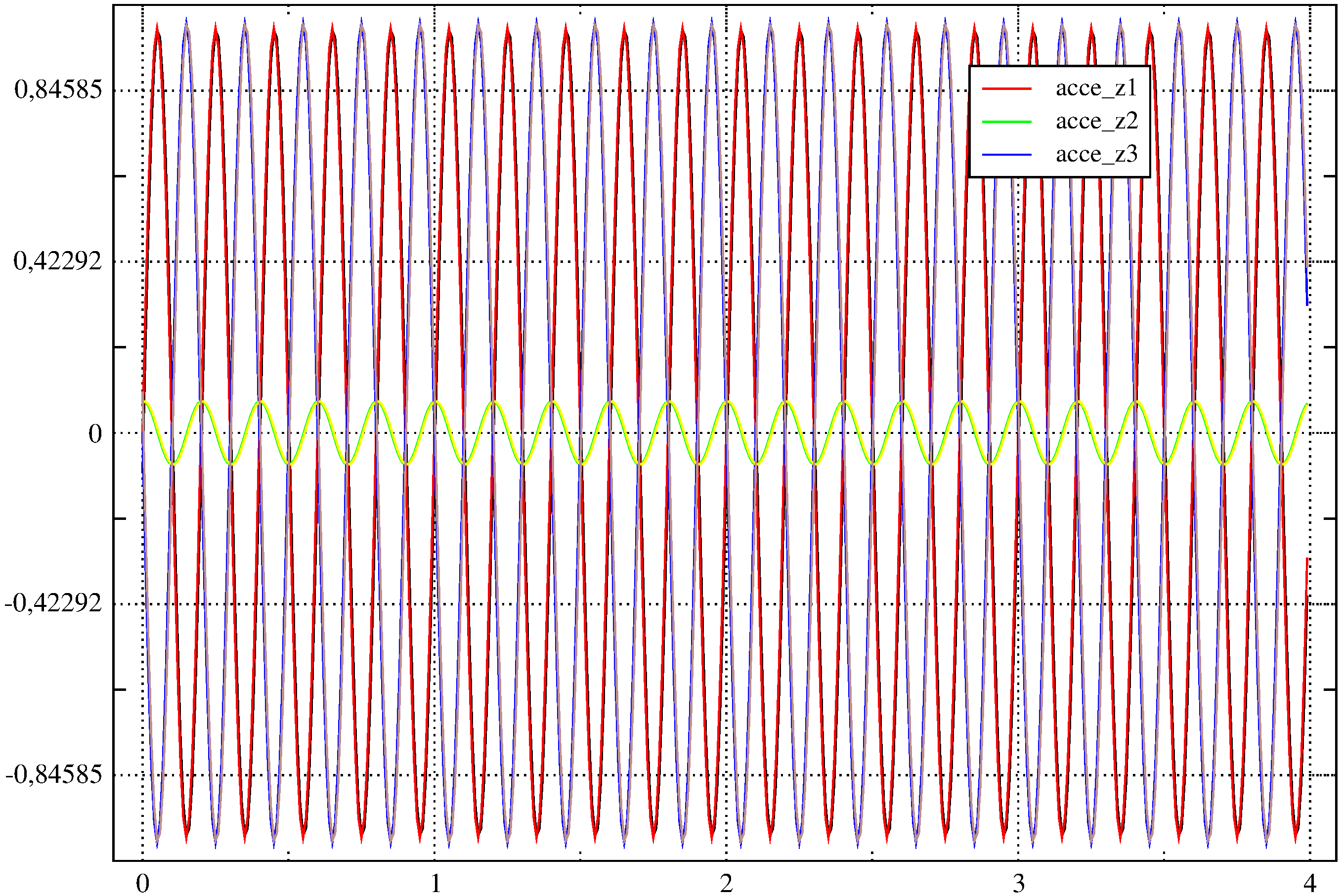
Acceleration \(\mathit{AZ}\), Point \(\mathit{NC}1\) \((\mathrm{50,}\mathrm{0,}0)\), \(T=\mathrm{0.05s}\) |
0.99503686 |
“AUTRE_ASTER” |
0.1% |
0.1% |
Acceleration \(\mathit{AZ}\), Point \(\mathit{NC2}\) \((\mathrm{50,}\mathrm{0,}–12.5)\), \(T=\mathrm{0.20s}\) |
0.077163903 |
“AUTRE_ASTER” |
0.1% |
|
AZ acceleration, Point \(\mathit{NC3}\) \((\mathrm{50,}\mathrm{0,}–25.0)\), \(T=\mathrm{0.05s}\) |
-1.0069431 |
“AUTRE_ASTER” |
0.1% |
3.5. Summary of the results of the C modeling#
The results are very similar (cf. superposition of the curves) to those obtained previously with the old operator MACRO_MISS_3D. There is a very slight phase difference.
The amplitudes are very similar, taking the values at the given times, the difference is of the order of 1%.
It is also observed that the results are the same with accelerograms on a time basis or on a frequency basis.
Comparison with solution MACRO_MISS_3D