3. Modeling A#
3.1. Read files#
Accelerogram SEPTEN not centered on unit 19.
Doearthquake accelerogram centered on unit 20.
3.2. Test and calculation#
for each signal read:
search for the max value,
calculation of the oscillator spectrum.
SPEC_OSCI NATURE: “OCCC” NATURE: “DEPL” or “ACCE” NORME: 1. /g or 1.
3.3. Tested sizes and results#
Identification |
Reference |
% tolerance |
Max amplitude accelerogram 1 \(t=7.935\) |
—0.638 |
0.1 |
oscillator spectrum 1 (not centered) \(\mathrm{freq.}100\) acceleration displacement |
6.258778 1.61607288E-06 |
0.1 0.1 |
max amplitude accelerogram 2 \(t=3.1\) |
1.0 |
0.1 |
oscillator spectrum 2 (centered) \(\mathrm{freq.}100\) |
1.0 |
0.1 |
3.4. notes#
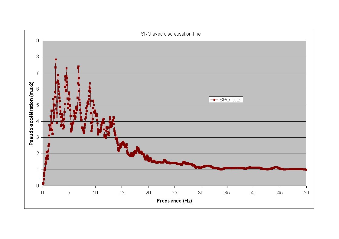
The precision of integration of the oscillator spectrum is not always satisfactory with the frequency list by default (on the asymptotic value, the deviation from the reference solution reaches almost 10%). Indeed, this list cuts to \(\mathrm{35,5}\mathrm{Hz}\), while the input signal has a significant frequency content up to more than \(50\mathrm{Hz}\)… As can be seen in the figure below (spectrum 2):
In general, the user is strongly advised to always check the frequency content (cutoff frequency, sampling) of the signal to be processed beforehand. Thus, it will then be possible to adapt the frequency list as best as possible for calculating the oscillator spectrum.
This test case is precisely the example for which it is necessary to broaden the frequency range, in order to properly capture the high frequencies of the input signal.
In practice, a list of frequencies ranging from \(\mathrm{0,1}\mathrm{Hz}\) to \(100\mathrm{Hz}\) is defined in steps of \(\mathrm{0,05}\mathrm{Hz}\), which will be used to calculate the oscillator spectrum. The deviation from the reference value for the asymptote of the pseudo-acceleration then becomes less than 0.02%.
All of these attributes of the functions read or created are tested and accurate.