3. Operands#

3.1. Operand MATER#

♦ MATER = mat [subdue]

This keyword allows you to enter the name of the material defined by DEFI_MATERIAU [U4.43.01], where the parameters necessary for the chosen behavior are provided.

3.2. Keyword COMPORTEMENT#

The syntax for this keyword is described in document [U4.51.11].

As part of this macro-command, the use of the operand RELATIONdu keyword COMPORTEMENTest is limited to the following elastoplastic soil laws:

“MOHR_COULOMB”
“MohrCoulombas”
“CAM_CLAY”
“CJS”
“DRUCK_PRAGER”
“DRUCK_PRAG_N_A”
“HUJEUX”
“Iwan”
“MFRONT”
“NLH_CSRM”
“MCC”
“CSSM”

3.3. Keyword CONVERGENCE#

◊ CONVERGENCE = _F ()

If neither of the following two operands is present, then everything is as follows: RESI_GLOB_RELA = 1.E-6

3.3.1. Operand RESI_GLOB_RELA/RESI_GLOB_MAXI#

◊ | RESI_GLOB_RELA = resi_real [R]

The algorithm continues global iterations as long as:

math:: underset {i=mathrm {1,}mathrm {1,}mathit {nbddl}}} {mathit {max}} | {F} _ {i} ^ {n} |phantom {rule {2em} {2em} {0ex}} |phantom {rule {max}} | {F} _ {i} ^ {n} |phantom {rule {2em} {0ex}} |phantom {rule {2em} {0ex}}}text {resi_rela}timesrule {2em} {0ex}} >phantom {rule {2em} {0ex}}}text {resi_rela}timesrule {2em} {0ex}} |L|

where \({F}^{n}\) is the residue of iteration \(n\) and \(L\) is the vector of the imposed load and the support reactions (Cf. [R5.03.01] for more details).

When the loading and the support reactions become zero, i.e. when \(L\) is zero (for example in the case of a total discharge), we try to pass from the relative convergence criterion RESI_GLOB_RELA to the absolute convergence criterion RESI_GLOB_MAXI. This operation is transparent for the user (alarm message sent in the.mess file). When the vector \(L\) becomes different from zero again, we automatically go back to the relative convergence criterion RESI_GLOB_RELA.

However, this failover mechanism cannot work at the first step of time. Indeed, to find a reasonable value of RESI_GLOB_MAXI automatically (since the user did not enter it), we need to have had at least one step converged on the RESI_GLOB_RELA mode. Therefore, if the load is zero from the first moment, the calculation stops. The user must then already check that the zero load is normal from the point of view of the modeling he is doing, and if this is the case, find another convergence criterion (RESI_GLOB_MAXI for example).

If this operand is not present, the test is performed with the value by default, unless RESI_GLOB_MAXI is present.

◊ | RESI_GLOB_MAXI = resi_max [R]

The algorithm continues global iterations as long as:

math:: underset {i=mathrm {1,}mathrm {1,}mathit {nbddl}}} {mathit {max}} | {F} _ {i} ^ {n} |phantom {rule {2em} {2em} {0ex}} |phantom {rule {2em}}}text {resi_maxi} |phantom {rule {2em} {2em} {0ex}} |phantom {rule {2em} {2em} {0ex}}text {resi_maxi}}

where \({F}^{n}\) is the residue from iteration \(n\) (see [R5.03.01] for more details). If this operand is absent, the test is not performed.

If both RESI_GLOB_RELA and RESI_GLOB_MAXI are present, both tests are performed.

3.3.2. Operand ITER_GLOB_MAXI#

◊ ITER_GLOB_MAXI = | 10 [DEFAULT]

| nb_iter

Maximum number of iterations performed to solve the global problem at any given time.

3.4. Keyword ESSAI_TRIA_DR_M_D#

This keyword factor (repeatable) makes it possible to perform a series of simulations of the same monotonous drained triaxial test with imposed deformation for which the loading parameters are varied (confinement pressure and imposed axial deformation), to post-process the results obtained and to write them in the form of graphs (in xmgrace format) and/or tables.

3.4.1. Entry and exit sign agreement#

The sign convention of geomechanics applies to the input parameters for imposed stresses or deformations, i.e. the values are positive in compression.

This convention also applies to predefined output variables, the complete list of which for this test is as follows:

INST: instant
EPS_AXI: axial deformation
EPS_LAT: lateral deformation
EPS_VOL: volume deformation
SIG_AXI: effective axial stress
SIG_LAT: effective lateral stress
P: average effective stress
Q: constraint deviator

However, this convention does not apply to non-predefined variables requested as output in NOM_CMP (§ 3.4.6).

3.4.2. Operands PRES_CONF, EPSI_IMPOSE, NB_INST#

♦ PRES_CONF = l_sigma_conf [L_r]

♦ EPSI_IMPOSE = l_epsi_impo [L_r]

◊ NB_INST = | 100 [DEFAULT]

| nbinst [I]

The PRES_CONF operand defines the list of confinement pressures that will be maintained during each test. Likewise, the EPSI_IMPOSE operand makes it possible to define the list of the final values of the compression load (imposed axial deformation ramp).

For this test, a final value for the axial strain ramp is assigned to each confinement pressure (see figure): lists PRES_CONF and EPSI_IMPOSE must therefore have the same cardinal value. This cardinal corresponds to the number of simulations that will be run under this keyword factor.

Since stresses and deformations are counted positively in compression, the values entered for PRES_CONF must be strictly positive. The values specified in EPSI_IMPOSE are strictly positive or negative, with a negative value indicating a loading in extension.

The NB_INSTpermet operand defines the loading time discretization (see figure), with a default value of 100 loading steps during the ramp.

.. image:: images/Cadre5.gif

.. _RefSchema_Cadre5.gif:

Figure 3.4.2-a: discretization and loading speed for the keywords ESSAI_TD and ESSAI_TND

3.4.3. Operand KZERO#

◊ KZERO = | 1 [DEFAULT]

kzero [R]

Value of the coefficient of the land at rest, allows to define an anisotropic confinement state: \({\mathrm{\sigma }}_{\mathit{xx}}={\mathrm{\sigma }}_{\mathit{yy}}={K}_{0}{\mathrm{\sigma }}_{\mathit{zz}}={K}_{0}\times \text{PRES\_CONF}\)

Note: When the value of KZEROest entered is different from 1, the actual confinement pressure of the test is no longer PRES_CONF, it becomes:

\({P}_{c}=\frac{1+2{K}_{0}}{3}\times \text{PRES\_CONF}\)

3.4.4. Operand TABLE_RESU#

◊ TABLE_RESU = l_tabres [L_co]

This optional operand makes it possible to give the list of the names of the concepts produced by the macro-command which will then be of type [table]. Each table produced contains the raw and post-processed results of a test simulation: list TABLE_RESU must therefore have the same cardinal value as lists PRES_CONF and EPSI_IMPOSE.

The title of each table produced is completed by the macro command, it includes:

the name of the keyword factor (here ESSAI_TRIA_DR_M_D) and its occurrence number (this one being repeatable);
the pair of values (PRES_CONF, EPSI_IMPOSE) characterizing the test load;

Example:

TABRES1 =CO (“TRES1”)

TABRES2 =CO (“TRES2”)

TABRES3 =CO (“TRES3”)

CALC_ESSAI_GEOMECA (

ESSAI_TRIA_DR_M_D = _F (

PRES_CONF = (-1.E4, -1. 5E4, -2.E4),

EPSI_IMPOSE = (-1.E-2, -1.E-2, -1.E-2),

TABLE_RESU = (TABRES1, TABRES2, TABRES3),),

);

TABRES1, TABRES2, and TABRES3sont filled in successively according to the order of lists PRES_CONF and EPSI_IMPOSE, the table below specifies the test results contained in each table.

EPSI_IMPOSE®	-1.0E-2	-1.0E-2	-1.0E-2
PRES_CONF	-1.0E-2	-1.0E-2	-1.0E-2
-1. 0E4	TABRES1
-1. 5E4		TABRES2
-2. 0E4			TABRES3

3.4.5. Operand GRAPHIQUE, PREFIXE_FICHIER#

◊ GRAPH = | ('P-Q', 'EPS_AXI-Q', 'EPS_AXI-EPS_VOL',

'P- EPS_VOL ') [DEFAUT]

| l_graph [l_KN]

This operand makes it possible to specify the types of graphics produced by the macro command. These graphs summarize the results of simulations run under the keyword current factor. A list by default is proposed. However, it is possible to bring up any graph by giving the desired combinations of components existing in the graph, in the form: ABSC - ORDO. The dash « - » separates the component requested on the x-axis from the component requested on the y-axis.

Example:

l_graph = (“P-Q”, “EPS_AXI -Q”,” INST - EPS_VOL “,” INST -V23”)

The non-predefined component V23 (corresponding to the plastic volume deformation of Hujeux’s law [R7.01.23]) must be declared in NOM_CMP (§ 3.4.6) to be taken into account. Otherwise, the requested graph is not brought up.

As for the predefined components whose complete list is given in § 3.4.1, they will possibly be displayed with the sign convention of the geomechanics, i.e. with positive values in compression.

In addition, all the components requested for graphic construction will be displayed in the output tables (§ 3.4.4).

The files containing these graphics are written in xmgrace format in the same directory specified by the user (type repeen result in astk), and are named as follows:

“prefix’_’test_name” _’occurence number’_’absc-ordo”.agr

A prefix can be added to the output file name using the optional keyword:

◊ PREFIXE_FICHIER = prefix [Kn]

3.4.6. Operand NOM_CMP#

◊ NOM_CMP = l_component [L_kn]

list of non-predefined components requested as output. These are all the existing components contained in fields SIGM, EPSI, and VARI produced by the calculation. These non-predefined components will be produced with the sign convention by default, i.e. with negative values when compressed.

Non-existing components are ignored.

3.4.7. Operand TABLE_REF#

◊ TABLE_REF = l_tabref [l_table]

This operand makes it possible to fill in reference curves (for example, experimental) tabulated and stored in the form of tables, in order to superimpose them on the curves resulting from simulations run under the keyword factor current. These reference curves are then included in the files produced by the GRAPHIQUE keyword.

Each table in list TABLE_REF must be created in advance using the CREA_TABLE [U4.33.02] operator, and formatted as follows:

tabref = CREA_TABLE (

LISTE = (_F (PARA = “TYPE”, LISTE_K = [typgraph,]),

_F (PARA = “LEGENDE”, LISTE_K = [malegend,]),

_F (PARA = “ABSCISSE”, LISTE_R = l_absc),

_F (PARA = “ORDONNEE”, LISTE_R = l_ordo),),);

with:

typgraph a character string whose value must belong to the list of values by default for the GRAPHIQUE keyword. This value makes it possible to identify the type of graph (and therefore the file) to which the reference curve should be added.
malegend a character string that contains the legend associated with the reference curve
l_absc and l_ordo are Python lists of real numbers containing the abscissa and the ordinates of the points of the reference curve respectively. These lists must therefore have even cardinal

3.4.8. Operands COULEUR, MARQUEUR, STYLE#

◊ COULEUR = l_color [L_i]

◊ MARQUEUR = l_marker [L_i]

◊ STYLE = l_style [L_i]

These operands accept a list of integers to define respectively the color, the type of marker, and the style of the curves displayed in the graphs. The information coded by each integer is given in the documentation on XMGRACE U2.51.01. The length of the list should be equal to that of PRES_CONF.

3.5. Keyword ESSAI_TRIA_ND_M_D#

This keyword factor (repeatable) makes it possible to perform a series of simulations of the same monotonous undrained triaxial test with imposed deformation (total saturation is assumed) for which the loading parameters (confinement pressure and imposed axial deformation) are varied, to post-process the results obtained and to write them in the form of graphs (in xmgrace format) and/or tables.

3.5.1. Entry and exit sign agreement#

The sign convention of geomechanics applies to the input parameters for imposed stresses or deformations, i.e. the values are positive in compression.

This convention also applies to predefined output variables, the complete list of which is as follows:

INST: instant
EPS_AXI: axial deformation
EPS_LAT: lateral deformation
EPS_VOL: volume deformation
SIG_AXI: effective axial stress
SIG_LAT: effective lateral stress
P: average effective stress
Q: constraint deviator
PRE_EAU: interstitial pressure

However, this convention does not apply to non-predefined variables requested as output in NOM_CMP (§ 3.5.7).

3.5.2. Operands PRES_CONF, EPSI_IMPOSE, NB_INST#

♦ PRES_CONF = l_sigma_conf [L_r]

♦ EPSI_IMPOSE = l_epsi_impo [L_r]

◊ NB_INST = | 100 [DEFAULT]

| nbinst [I]

Same as in § 3.4.2.

3.5.3. Operand BIOT_COEF#

◊ BIOT_COEF = | 1 [DEFAULT]

| Biot [R]

Value of the Biot coefficient.

3.5.4. Operand KZERO#

◊ KZERO = | 1 [DEFAULT]

kzero [R]

Same as in § 3.4.3.

3.5.5. Operand TABLE_RESU#

◊ TABLE_RESU = l_tabres [L_co]

Same as in § 3.4.4.

3.5.6. Operand GRAPHIQUE, PREFIXE_FICHIER#

◊ GRAPH = | ('P-Q', 'EPS_AXI-Q',

'EPS_AXI - PRE_EAU') [DEFAUT]

| l_graph [l_KN]

◊ PREFIXE_FICHIER = prefix [Kn]

Same as in § 3.4.5.

3.5.7. Operand NOM_CMP#

◊ NOM_CMP = l_component [L_kn]

Same as in § 3.4.6.

3.5.8. Operand TABLE_REF#

◊ TABLE_REF = l_tabref [l_table]

Same as in § 3.4.7.

3.5.9. Operands COULEUR, MARQUEUR, STYLE#

◊ COULEUR = l_color [L_i]

◊ MARQUEUR = l_marker [L_i]

◊ STYLE = l_style [L_i]

Same as in § 3.4.8.

3.6. Keyword ESSAI_CISA_DR_C_D#

This keyword factor (repeatable) makes it possible to perform a series of simulations of the same drained cyclic shear test with imposed shear deformation for which the loading parameters are varied (confinement pressure, amplitude of shear deformation and number of cycles), to post-process the results obtained and to write them in the form of graphs (in xmgrace format) and/or tables.

3.6.1. Entry and exit sign agreement#

The sign convention of geomechanics applies to the input parameters for imposed stresses or deformations, i.e. the values are positive in compression.

This convention also applies to predefined output variables. However, this convention does not apply to non-predefined variables requested as output in NOM_CMP (§ 3.6.7).

In this test, a distinction is made between pre-defined level 2 output variables that correspond to the variables produced by the test, the complete list of which is as follows:

INST: instant
GAMMA: shear deformation \(\mathrm{\gamma }=2{\mathrm{ϵ}}_{\mathit{xy}}\)
SIG_XY: shear stress

And the pre-defined level 1 output variables that correspond to curves whose points represent the result of a test (e.g. curve \(\frac{G}{{G}_{\text{max}}}-\mathrm{\gamma }\)). The complete list of Level 1 variables is as follows:

G_SUR_GMAX: \(\frac{G}{{G}_{\text{max}}}\)
DAMPING: hysteretic damping \(\frac{\mathrm{\Delta }W}{\mathrm{\pi }W}\)

3.6.2. Operands PRES_CONF, GAMMA_IMPOSE, NB_CYCLE, NB_INST, TYPE_CHARGE#

♦ PRES_CONF = l_sigma_conf [L_r]

♦ GAMMA_IMPOSE = l_gamma_impo [L_r]

♦ NB_CYCLE = nbcyc [I]

◊ NB_INST = | 25 [DEFAULT]

|nbinst [I]

◊ CHARGE_TYPE = | 'SINUSOIDAL' [DEFAULT]

|'TRIANGULAR' [Kn]

These operands make it possible to define the load of each of the simulations to be run under the current keyword factor, as well as its discretization. Their meaning is summarized in the figure and detailed below:

PRES_CONF allows you to define the list of confinement pressures (strictly positive) that will be maintained during each test;
GAMMA_IMPOSE allows you to define the list of (strictly positive) amplitudes of shear deformation \(\gamma =2{\epsilon }_{\mathit{xy}}\) of the imposed cyclic load;
NB_CYCLEcorrespond to the number of cycles, fixed for all simulations.
NB_INSTpermet to define the time discretization of the load, and corresponds to the number of loading steps per quarter of a cycle
TYPE_CHARGE indicates the type of load required: sinusoidal or triangular;

For each PRES_CONF confinement pressure, we perform as many simulations as there are elements in list GAMMA_IMPOSE. Unlike essays TRIA_DR_M_Det TRIA_ND_M_D (see § 3.4 and § 3.5 respectively), these lists are not in bijection and there are in total

\(\mathit{card}(\text{PRES\_CONF})\times \mathit{card}(\text{GAMMA\_IMPOSE})\) simulations run.

Figure 3.6.2-a : discretization and rate of loading of the triangular type for the keyword ESSAI_CISA_DR_C_D for 3 loading cycles

3.6.3. Operand GAMMA_ELAS#

◊ GAMMA_ELAS = | 1.E-7 [DEFAULT]

|gamma_elas [R]

For each confinement pressure, the maximum secant shear modulus (i.e. healthy material) is determined by simulating an imposed shear deformation ramp (in terms of distortion) whose final value is GAMMA_ELAS. This value must be such that the material remains within its range of elasticity (linear or not, depending on the behavioral relationship used). GAMMA_ELAS is 1.E-7 by default, and any value entered by the user must be less than 1.E-7 by default. If the value entered does not allow you to remain in the elasticity domain, the code stops with a fatal error.

3.6.4. Operand KZERO#

◊ KZERO = | 1 [DEFAULT]

kzero [R]

Same as in § 3.4.3.

3.6.5. Operand TABLE_RESU#

◊ TABLE_RESU = l_tabres [L_co]

This optional operand makes it possible to give the list of the names of the concepts produced by the macro-command which will then be of type [table]. The size of this list should check:

\(\mathit{card}(\text{TABLE\_RESU})=\mathit{card}(\text{PRES\_CONF})+1\)

In fact, each table produced groups together the raw results of all the simulations executed for the same confinement pressure (PRES_CONF), in which each simulation corresponds to a pack of contiguous columns whose titles are all indexed by the same integer (index of the value considered in the list GAMMA_IMPOSE). An additional table summarizing the post-treatments carried out at the end of all the simulations is also produced. This table contains for each confinement pressure (PRES_CONF) the values of the standardized secant shear modulus \(\frac{G}{{G}_{\mathit{max}}}\) and of the hysteretic damping ratio \(\frac{\mathrm{\Delta }W}{\mathrm{\pi }W}\) facing each other with the amplitudes of imposed distortion (GAMMA_IMPOSE). Hysteretic damping \(\frac{\mathrm{\Delta }W}{\mathrm{\pi }W}\) for the last simulated cycle is calculated according to Kohusho [] in the following way (Figure):

\(\mathrm{\Delta }W={\int }_{C}\mathrm{\delta }{\mathrm{\sigma }}_{\mathit{xy}}\mathrm{\delta }\mathrm{\gamma }\) the area of the last hysteresis loop;
\(W=\mathrm{\Delta }{\mathrm{\sigma }}_{\mathit{xy}}\mathrm{\Delta }\mathrm{\gamma }\) the associated elastic energy

This table corresponds to the concept name given in the last position in list TABLE_RESU. Excerpts from these tables are shown in the example below.

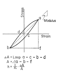
Figure 3.6.5-a: Definition of hysteretic damping according to Kokusho []

Example:

TABRES1 = CO (“TRES1”)

TABRES2 = CO (“TRES2”)

TABBILA = CO (“TBILA”)

CALC_ESSAI_GEOMECA (

ESSAI_CISA_DR_C_D = _F (

PRES_CONF = (1.E5, 2.0 5E5,),

GAMMA_IMPOSE = (1.E-5, 5.E-5, 1.E-5, 1.E-4, 1.E-3),

NB_CYCLE = 3,

TABLE_RESU = (TABRES1, TABRES2, TABBILA),),

);

For this example, the table below shows the simulation results contained in tables TABRES1et TABRES2, as well as the order in which these tables are filled.

GAMMA_IMPOSE	1.E-5	5.E-5	1.E-4	1.E-3
PRES_CONF	1.E-5	5.E-5	1.E-4	1.E-3
1.E5	TABRES1	TABRES1	TABRES1	TABRES1
2.0 5E5	TABRES2	TABRES2	TABRES2	TABRES2

Below is an extract from table TABRES1contenant showing the raw results of the simulations executed for the first value of PRES_CONF (TABRES2étant constructed in the same way, for the second value of PRES_CONF).

#——————————————————————————–

Raw #Resultats: ESSAI_CISA_C number 1/PRES_CONF = -1.000000E+05

GAMMA_IMPOSE_1 INST_1 GAMMA_1 SIG_XY_1 GAMMA_IMPOSE_2 INST_2 GAMMA_2 SIG_XY_2…

1.00000E-05 0.00000E+00 0.00000E+00 0.00000E+00 0.00000E+00 5.00000E-05 0.00000E+00 0.00000E+00 0.00000E+00 0.00000E+00…

4.00000E-01 -4.00000E-07 -3.79317E+01 - 4.00000E-01 -2.00000E-06 -1.89658E+02…
8.00000E-01 -8.00000E-07 -7.58633E+01 - 8.00000E-01 -4.00000E-06 -3.79317E+02…
1.20000E+00 -1.20000E-06 -1.13795E+02 - 1.20000E+00 -6.00000E-06 -5.50536E+02…
1.60000E+00 -1.60000E-06 -1.51727E+02 - 1.60000E+00 -8.00000E-06 -7.19697E+02…
2.00000E+00 -2.00000E-06 -1.89658E+02 - 2.00000E+00 -1.00000E-05 -8.88778E+02…
2.40000E+00 -2.40000E-06 -2.27590E+02 - 2.40000E+00 -1.20000E-05 -1.05778E+03…
2.80000E+00 -2.80000E-06 -2.65522E+02 - 2.80000E+00 -1.40000E-05 -1.22670E+03…
3.20000E+00 -3.20000E-06 -3.03453E+02 - 3.20000E+00 -1.60000E-05 -1.39554E+03…
3.60000E+00 -3.60000E-06 -3.41385E+02 - 3.60000E+00 -1.80000E-05 -1.56429E+03…
4.00000E+00 -4.00000E-06 -3.79317E+02 - 4.00000E+00 -2.00000E-05 -1.73297E+03…
4.40000E+00 -4.40000E-06 -4.15150E+02 - 4.40000E+00 -2.20000E-05 -1.90156E+03…
4.80000E+00 -4.80000E-06 -4.49001E+02 - 4.80000E+00 -2.40000E-05 -2.07007E+03…
5.20000E+00 -5.20000E-06 -4.82849E+02 - 5.20000E+00 -2.60000E-05 -2.23850E+03…
5.60000E+00 -5.60000E-06 -5.60000E-06 -5.16693E+02 - 5.60000E+00 -2.80000E-05 -2.40684E+03…
6.00000E+00 -6.00000E-06 -5.50535E+02 - 6.00000E+00 -3.00000E-05 -2.57510E+03…
6.40000E+00 -6.40000E-06 -5.84374E+02 - 6.40000E+00 -3.20000E-05 -2.74327E+03…
6.80000E+00 -6.80000E-06 -6.18209E+02 - 6.80000E+00 -3.40000E-05 -2.91136E+03…
7.20000E+00 -7.20000E-06 -6.52041E+02 - 7.20000E+00 -3.60000E-05 -3.07937E+03…
7.60000E+00 -7.60000E-06 -6.85870E+02 - 7.60000E+00 -3.80000E-05 -3.24729E+03…
8.00000E+00 -8.00000E-06 -7.19695E+02 - 8.00000E+00 -4.00000E-05 -3.41511E+03…
8.40000E+00 -8.40000E-06 -7.53517E+02 - 8.40000E+00 -4.20000E-05 -3.58284E+03…
8.80000E+00 -8.80000E-06 -7.87336E+02 - 8.80000E+00 -4.40000E-05 -3.75049E+03…
9.20000E+00 -9.20000E-06 -8.21152E+02 - 9.20000E+00 -4.60000E-05 -3.91805E+03…
9.60000E+00 -9.60000E-06 -8.54965E+02 - 9.60000E+00 -4.80000E-05 -4.08436E+03…
1.00000E+01 -1.00000E-05 -8.88774E+02 - 1.00000E+01 -5.00000E-05 -4.24698E+03…
1.04000E+01 -9.60000E-06 -8.50842E+02 - 1.04000E+01 -4.80000E-05 -4.05732E+03…
1.08000E+01 -9.20000E-06 -8.12911E+02 - 1.08000E+01 -4.60000E-05 -3.86767E+03…
1.12000E+01 -8.80000E-06 -7.74979E+02 - 1.12000E+01 -4.40000E-05 -3.67801E+03…
1.16000E+01 -8.40000E-06 -7.37047E+02 - 1.16000E+01 -4.20000E-05 -3.48835E+03…
1.20000E+01 -8.00000E-06 -6.99116E+02 - 1.20000E+01 -4.00000E-05 -3.31514E+03…
1.24000E+01 -7.60000E-06 -6.61184E+02 - 1.24000E+01 -3.80000E-05 -3.14591E+03…
1.28000E+01 -7.20000E-06 -6.23252E+02 - 1.28000E+01 -3.60000E-05 -2.97673E+03…
1.32000E+01 -6.80000E-06 -5.85321E+02 - 1.32000E+01 -3.40000E-05 -2.80759E+03…
1.36000E+01 -6.40000E-06 -5.47389E+02 - 1.36000E+01 -3.20000E-05 -2.63849E+03…
1.40000E+01 -6.00000E-06 -5.09458E+02 - 1.40000E+01 -3.00000E-05 -2.46942E+03…
1.44000E+01 -5.60000E-06 -4.71526E+02 - 1.44000E+01 -2.80000E-05 -2.30040E+03…
1.48000E+01 -5.20000E-06 -4.33594E+02 - 1.48000E+01 -2.60000E-05 -2.13142E+03…
1.52000E+01 -4.80000E-06 -3.95663E+02 - 1.52000E+01 -2.40000E-05 -1.96247E+03…
1.56000E+01 -4.40000E-06 -3.57731E+02 - 1.56000E+01 -2.20000E-05 -1.79357E+03…
1.60000E+01 -4.00000E-06 -3.19799E+02 - 1.60000E+01 -2.00000E-05 -1.62471E+03…
1.64000E+01 -3.60000E-06 -2.81868E+02 - 1.64000E+01 -1.80000E-05 -1.45589E+03…
1.68000E+01 -3.20000E-06 -2.43936E+02 - 1.68000E+01 -1.60000E-05 -1.28711E+03…
1.72000E+01 -2.80000E-06 -2.06004E+02 - 1.72000E+01 -1.40000E-05 -1.11836E+03…
1.76000E+01 -2.40000E-06 -1.68073E+02 - 1.76000E+01 -1.20000E-05 -9.49666E+02…
1.80000E+01 -2.00000E-06 -1.30141E+02 - 1.80000E+01 -1.00000E-05 -7.81009E+02…
1.84000E+01 -1.60000E-06 -9.23287E+01 - 1.84000E+01 -8.00000E-06 -6.12391E+02…

Below, the content of supplementary table TABBILA is also presented, summarizing the post-treatments (\(\frac{G}{{G}_{\mathit{max}}}\) and \(\mathit{DAMPING}\)) carried out at the end of all the simulations. Each pack of contiguous columns whose titles are indexed by the same integer (index of the value considered in list PRES_CONF) corresponds to the post-treatments carried out for the same confinement pressure.

#——————————————————————————–

Global #Resultats: ESSAI_CISA_C number 1

PRES_CONF_1 GAMMA_IMPOSE_1 G_SUR_GMAX_1 DAMPING_1 PRES_CONF_2 GAMMA_IMPOSE_2 G_SUR_GMAX_2 DAMPING_2

-1.00000E+05 1.00000E-05 9.37244E-01 1.79484E-02 -2.00000E+05 1.00000E-05 9.65623E-01 1.30248E-02

5.00000E-05 8.95847E-01 7.93301E-03 - 5.00000E-05 9.26152E-01 6.34512E-03
1.00000E-04 7.91534E-01 5.24988E-02 - 1.00000E-04 8.82990E-01 2.26809E-02
1.00000E-03 2.81687E-01 2.16980E-01 - 1.00000E-03 3.69590E-01 1.89750E-01

3.6.6. Operand GRAPHIQUE, PREFIXE_FICHIER#

◊ GRAPH = | ('GAMMA-SIG_XY', 'GAMMA-G_SUR_GMAX',

'GAMMA - DAMPING',

'G_SUR_GMAX - DAMPING') [DEFAUT]

| l_graph [L_kn]

◊ PREFIXE_FICHIER = prefix [Kn]

Same as in § 3.4.5, except that unlike level 2 charts, which can be any, level 1 charts are to be selected from the list:

“GAMMA - G_SUR_GMAX”;
“GAMMA - DAMPING”;
“G_SUR_GMAX - DAMPING”

3.6.7. Operand NOM_CMP#

◊ NOM_CMP = l_component [L_kn]

Same as in § 3.4.6.

3.6.8. Operand TABLE_REF#

◊ TABLE_REF = l_tabref [l_table]

Same as in § 3.4.7.

3.6.9. Operands COULEUR_NIV1, MARQUEUR_NIV1, STYLE_NIV1, COULEUR_NIV2,, MARQUEUR_NIV2, STYLE_NIV2#

◊ COULEUR_NIV1 = l_color_lev1 [L_i]

◊ MARQUEUR_NIV1 = l_marker_lev1 [L_i]

◊ STYLE_NIV1 = l_style_lev1 [L_i]

◊ COULEUR_NIV2 = l_color_lev2 [L_i]

◊ MARQUEUR_NIV2 = l_marker-lev2 [L_i]

◊ STYLE_NIV2 = l_style_niv2 [L_i]

These operands accept a list of integers to define respectively the color, the type of marker, and the style of the curves displayed in the graphs. The information encoded by each integer is given in the documentation on XMGRACEU2 .51.01. The length of the level 1 list should be equal to the length of PRES_CONF. The length of the level 2 list should be equal to the length of GAMMA_IMPOSE.

3.7. Keyword ESSAI_TRIA_ND_C_F#

This keyword factor (repeatable) makes it possible to perform a series of simulations of the same undrained triaxial test (total saturation is assumed) cyclic at an imposed force for which the loading parameters are varied (confinement pressure, magnitude of effective axial stress imposed, and number of cycles), to post-process the results obtained and to write them in the form of graphs (in xmgrace format) and/or tables.

3.7.1. Entry and exit sign agreement#

The sign convention of geomechanics applies to the input parameters for imposed stresses or deformations, i.e. the values are positive in compression.

This convention also applies to predefined output variables. However, this convention does not apply to non-predefined variables requested as output in NOM_CMP (§ 3.7.9).

In this test, a distinction is made between pre-defined level 2 output variables that correspond to the variables produced by the test, the complete list of which is as follows:

INST: instant
EPS_AXI: axial deformation
EPS_LAT: lateral deformation
EPS_VOL: volume deformation
SIG_AXI: effective axial stress
SIG_LAT: effective lateral stress
P: average effective stress
Q: constraint deviator
PRE_EAU: interstitial pressure
RU: pore pressure coefficient equal to \({r}_{u}=\frac{3}{1+2{K}_{0}}\frac{\mathrm{\Delta }{u}_{w}}{\mathrm{\sigma }{\text{'}}_{v\mathrm{,0}}}\)

And the pre-defined level 1 output variables that correspond to curves whose points represent the result of a test (e.g. curve \(\mathit{CRR}-{N}_{\mathit{cyc}}\)). The complete list of Level 1 variables is as follows:

NCYCL: number of cycles from loading to liquefaction
DSIGM: maximum imposed stress normalized by the initial average effective stress \(\mathit{DSIGM}=\mathit{CRR}=\frac{{Q}_{\text{max}}}{P{\text{'}}_{0}}\)

3.7.2. Operands PRES_CONF, SIGM_IMPOSE, NB_CYCLE, NB_INST,, NB_INST_MONO, TYPE_CHARGE#

♦ PRES_CONF = l_sigma_conf [L_r]

♦ SIGM_IMPOSE = l_sigma_impo [L_r]

♦ NB_CYCLE = nbcyc [I]

◊ NB_INST = | 25 [DEFAULT]

| nbinst [I]

◊ NB_INST_MONO= | 400 [DEFAULT]

| nbinst_mono [I]

◊ CHARGE_TYPE = | 'SINUSOIDAL' [DEFAULT]

|'TRIANGULAR' [Kn]

PRES_CONF allows you to define the list of confinement pressures (strictly positive) that will be maintained during each test;
SIGM_IMPOSE allows you to define the list of effective axial stress amplitudes of the imposed cyclic load (with PRES_CONF the average stress). A strictly positive value indicates a first load in compression, a strictly negative value indicates a first load in extension;
NB_CYCLEcorrespond to the number of cycles, fixed for all simulations;
NB_INSTpermet to define the time discretization of loading, and corresponds to the number of loading steps per quarter of a cycle;
NB_INST_MONO makes it possible to define the temporal discretization of monotonic loads with imposed deformation after detecting instability, and corresponds to the number of loading steps per quarter of a cycle. The number of moments must be sufficiently large (>100) for a sufficiently accurate detection of the achievement of the force setpoint;
TYPE_CHARGE indicates the type of load required: sinusoidal or triangular;

For each PRES_CONF confinement pressure, we perform as many simulations as there are elements in list SIGM_IMPOSE. Unlike essays TRIA_DR_M_Det TRIA_ND_M_D (see § 3.4 and § 3.5 respectively), these lists are not in bijection and there are in total:

\(\mathit{card}(\text{PRES\_CONF})\times \mathit{card}(\text{SIGM\_IMPOSE})\) simulations run.

Figure 3.7.2-a: discretization and shape of the triangular load for the keyword ESSAI_TRIA_ND_C_D for 3 loading cycles

Note:

For loose sands, the stress control of the test poses difficulties when crossing the two instability lines, represented in blue in Figure. In fact, the imposition of a maximum stress setpoint greater than the maximum allowable stress on the instability line leads either to a discrepancy or to a false solution (sudden jump in stress visible in Figure ). In fact, the instability line represents the location of all the maximum allowable constraints of a trial TRIA_ND_M_D monotonic for different initial consolidation values (black curve) .

The problem does not arise for dense sand, because there are no maximum constraints in this case, as can be seen from the black curve in Figure .

For this test, there is therefore an automatic procedure **for managing unstable situations. It consists in detecting the instability and continuing the test under controlled deformation. The detection criteria are as follows:*

non-convergence of the calculation

\(\frac{\Delta Q}{\Delta P}<0.25\) and \(\frac{\mathrm{\Delta }{\mathrm{ϵ}}_{\mathit{zz}}^{\text{+}}}{\mathrm{\Delta }{\mathrm{ϵ}}_{\mathit{zz}}^{\text{-}}}>10\)

We continue with the number of remaining cycles by a series of tests TRIA_ND_M_D monotonic with controlled deformation, at the rate of two tests per cycle ( \(\pm {\mathrm{ϵ}}_{\mathit{max}}\) to reach \(\pm {\sigma }_{\mathit{max}}\) ). The maximum deformation sett \({\mathrm{ϵ}}_{\mathit{max}}\) imposed is 4%, or 12% if the previous setpoint was insufficient. The list of times for these tests TRIA_ND_M_D ranges from 0 to 100 seconds in steps of 0.2 seconds (or 0.1 seconds if the setpoint is \({\mathrm{ϵ}}_{\mathit{max}}=12\text{\%}\) ) .

The sequence of one test TRIA_ND_M_D with controlled deformation to the other is carried out by restarting the calculation from the last moment when the stress setting \(\pm {\sigma }_{\mathit{max}}\) is reached.

In Figure , an example of loose sand (test case comp012c) shows the solution obtained with or without the instability management procedure.

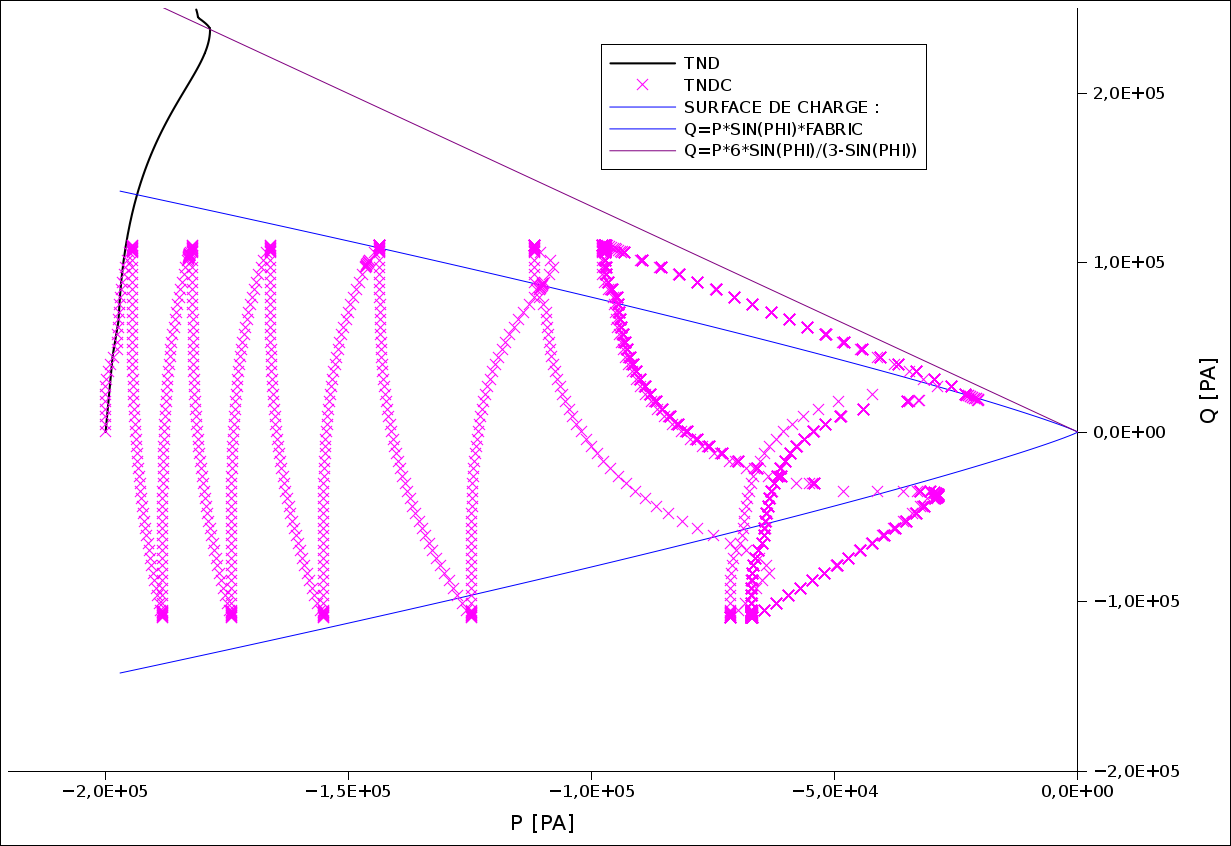
Figure 3.7.2-b: Result of the TRIA_ND_M_D (black) and TRIA_ND_C_F (pink) tests for dense sand. The failure state is represented by the purple line, and the instability lines are blue.

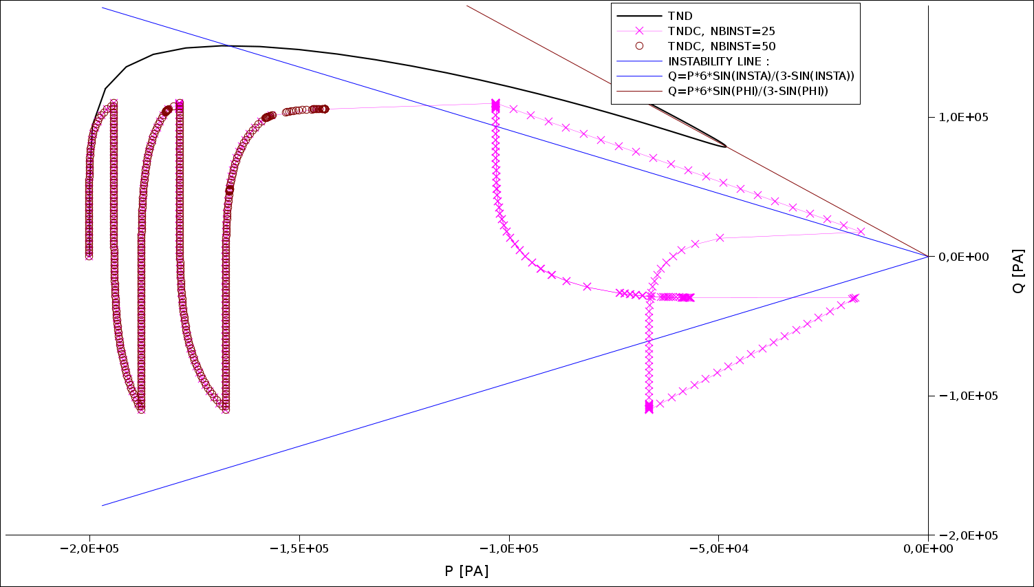
Figure 3.7.2-c :: **Test result* TRIA_ND_M_D (black) and TRIA_ND_C_F * (pink) for loose sand. The failure state is represented by the purple line, and the instability lines are blue.

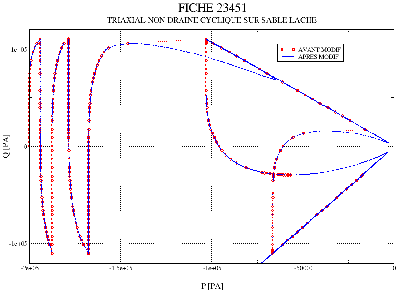
Figure 3.7.2-d : Test result TRIA_ND_C_F: **Test result* * for loose sand with (blue) or without (red) the instability management procedure.

3.7.3. Operand CRIT_LIQUEFACTION, VALE_CRIT, ARRET_LIQUEFACTION#

♦ CRIT_LIQUEFACTION = (“RU_MAX”, “EPSI_ABSO_MAX”,

“EPSI_RELA_MAX”)

♦ VALE_CRIT = l_vale [L_r]

◊ ARRET_LIQUEFACTION = | “YES” [DEFAULT]

|'NO'

Maximum value of the liquefaction criterion, to be compared with: \({r}_{u}=∣\frac{u}{{P}_{0}}∣\)

In CRIT_LIQUEFACTION, we choose a combination of criteria from the following list:

RU_MAXcorrespond with the liquefaction coefficient equal to \({r}_{u}=\frac{3}{1+2{K}_{0}}\frac{\mathrm{\Delta }{u}_{w}}{\mathrm{\sigma }{\text{'}}_{v\mathrm{,0}}}\), necessarily between \(\left]0,1\right]\) (Figure);
EPSI_ABSO_MAX corresponds to the axial deformation threshold called « single amplitude », positive in compression and negative in extension in the interval \(\left]-5,5\right]\phantom{\rule{2em}{0ex}}(\text{\%})\) (Figure);
EPSI_RELA_MAX corresponds to the criterion in terms of axial deformation amplitude over a period, called « double amplitude », which is necessarily positive and less than 5% (Figure);

The list of values, with the same cardinal value, is given in VALE_CRIT. The order of the criteria should correspond to the order of the numerical values.

If several criteria are chosen, liquefaction is stipulated to take place when all the criteria have been met in succession. The calculation is stopped at the last cycle where the last criterion is met, if possible, if ARRET_LIQUEFACTION = “OUI”. If ARRET_LIQUEFACTION = “NON”, the test is continued until the number of cycles specified in NB_CYCLE.

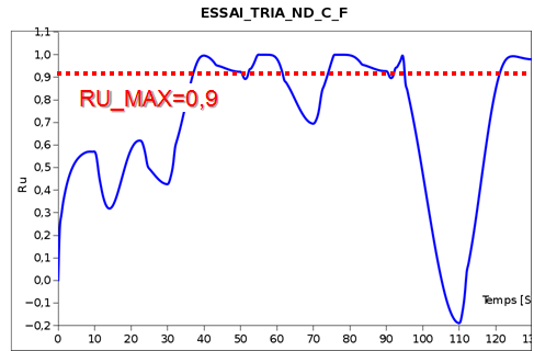
Figure 3.7.3-a : Criterion RU_MAX =0.9

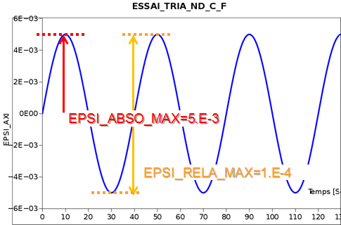
Figure 3.7.3-b : Criteria EPSI_ABSO_MAX = 5E-3 and EPSI_RELA_MAX = 1E-4

3.7.4. Operand BIOT_COEF#

◊ BIOT_COEF = | 1 [DEFAULT]

| Biot [R]

Value of the Biot coefficient.

3.7.5. Operand KZERO#

◊ KZERO = | 1 [DEFAULT]

kzero [R]

Same as in § 3.4.3.

3.7.6. Operand UN_SUR_K#

♦ UN_SUR_K = unsurk [R]

Value of the inverse of the compressibility modulus of water.

3.7.7. Operand TABLE_RESU#

◊ TABLE_RESU = l_tabres [L_co]

This optional operand makes it possible to give the list of the names of the concepts produced by the macro-command which will then be of type [table]. The size of this list should check:

\(\mathit{card}(\text{TABLE\_RESU})=\mathit{card}(\text{PRES\_CONF})+1\)

In fact, each table produced groups together the raw results of all the simulations executed for the same confinement pressure (PRES_CONF), in which each simulation corresponds to a pack of contiguous columns whose titles are all indexed by the same integer (index of the value considered in the list SIGM_IMPOSE). An additional table summarizing the post-treatments carried out at the end of all the simulations is also produced. This table contains for each confinement pressure (PRES_CONF) the number of cycles at the end of which the soil liquefaction criterion has been reached NCYCL, facing each other with the amplitudes of effective imposed stress (SIGM_IMPOSE). Liquefaction is considered to take place when all the criteria selected in paragraph § 3.7.3 are met in succession.

This table corresponds to the concept name given in the last position in list TABLE_RESU. Excerpts from these tables are shown in the example below.

Example:

TABRES1 =CO (“TRES1”)

TABRES2 =CO (“TRES2”)

TABRES3 =CO (“TRES3”)

TABBILA =CO (“TBILA”)

CALC_ESSAI_GEOMECA (

ESSAI_TRIA_ND_C_F = _F (

PRES_CONF = (3.E4, 3.2 5E4, 3. 5E4),

SIGM_IMPOSE = (1.E4, 1. 1E4, 1. 2E4, 1. 3E4, 1. 6E4),

UN_SUR_K = 1.E-12,

TABLE_RESU = (TABRES1, TABRES2, TABRES3, TABBILA)),

);

For this example, the table below shows the simulation results contained in tables TABRES1, TABRES2, and TABRES3, as well as the order in which these tables are filled.

SIGM_IMPOSE	1.E4	1.1E4	1.2E4	1.3E4	1.6E4
PRES_CONF Could You	1.E4	1.1E4	1.2E4	1.3E4	1.6E4
3.E4	TABRES1	TABRES1	TABRES1	TABRES1	TABRES1
3.2 5E4	TABRES2	TABRES2	TABRES2	TABRES2	TABRES2
3.5E4	TABRES3	TABRES3	TABRES3	TABRES3	TABRES3

Below is an extract from table TABRES2 containing the raw results of the simulations run for the second value of PRES_CONF.

#——————————————————————————–

Raw #Resultats: ESSAI_TND_C number 1/PRES_CONF = -3.250000E+04

SIGM_IMPOSE_1 INST_1 EPS_AXI_1 EPS_LAT_1… PRE_EAU_1 SIGM_IMPOSE_2 INST_2…

1.00000E+04 0.00000E+00 0.00000E+00 0.00000E+00 0.00000E+00… -0.00000E+00 1.10000E+04 0.00000E+00…

4.00000E-01 2.37788E-06 -1.18887E-06… -1.33316E+02 - 4.00000E-01…
8.00000E-01 5.27009E-06 -2.63491E-06… -2.66632E+02 - 8.00000E-01…
1.20000E+00 8.17434E-06 -4.08697E-06… -3.99948E+02 - 1.20000E+00…
1.60000E+00 1.10910E-05 -5.54522E-06… -5.33263E+02 - 1.60000E+00…
2.00000E+00 1.40203E-05 -7.00984E-06… -6.66579E+02 - 2.00000E+00…
2.40000E+00 1.69628E-05 -8.48101E-06… -7.99895E+02 - 2.40000E+00…
2.80000E+00 1.99187E-05 -9.95886E-06… -9.33211E+02 - 2.80000E+00…
3.20000E+00 2.30002E-05 -1.14996E-05… -1.06631E+03 - 3.20000E+00…
3.60000E+00 2.65689E-05 -1.32839E-05… -1.19796E+03 - 3.60000E+00…
4.00000E+00 3.06705E-05 -1.53346E-05… -1.32706E+03 - 4.00000E+00…
4.40000E+00 3.53282E-05 -1.76634E-05… -1.45247E+03 - 4.40000E+00…
4.80000E+00 4.05684E-05 -2.02834E-05… -1.57305E+03 - 4.80000E+00…
5.20000E+00 4.64193E-05 -2.32088E-05… -1.68756E+03 - 5.20000E+00…
5.60000E+00 5.29170E-05 -2.64576E-05… -1.79469E+03 - 5.60000E+00…
6.00000E+00 6.01011E-05 -3.00496E-05… -1.89303E+03 - 6.00000E+00…
6.40000E+00 6.80160E-05 -3.40070E-05… -1.98113E+03 - 6.40000E+00…
6.80000E+00 7.67173E-05 -3.83576E-05… -2.05731E+03 - 6.80000E+00…
7.20000E+00 8.62682E-05 -4.31330E-05… -2.11975E+03 - 7.20000E+00…
7.60000E+00 9.67455E-05 -4.83717E-05… -2.16636E+03 - 7.60000E+00…
8.00000E+00 1.08244E-04 -5.41211E-05… -2.19469E+03 - 8.00000E+00…
8.40000E+00 1.20878E-04 -6.04380E-05… -2.20193E+03 - 8.40000E+00…
8.80000E+00 1.34791E-04 -6.73947E-05… -2.18477E+03 - 8.80000E+00…
9.20000E+00 1.50170E-04 -7.50842E-05… -2.13899E+03 - 9.20000E+00…
9.60000E+00 1.67253E-04 -8.36253E-05… -2.05939E+03 - 9.60000E+00…
1.00000E+01 1.86360E-04 -9.31790E-05… -1.93918E+03 - 1.00000E+01…
1.04000E+01 1.84117E-04 -9.20575E-05… -1.80586E+03 - 1.04000E+01…
1.08000E+01 1.81336E-04 -9.06674E-05… -1.67255E+03 - 1.08000E+01…
1.12000E+01 1.78318E-04 -8.91580E-05… -1.53923E+03 - 1.12000E+01…
1.16000E+01 1.75296E-04 -8.76474E-05… -1.40592E+03 - 1.16000E+01…
1.20000E+01 1.72272E-04 -8.61353E-05… -1.27260E+03 - 1.20000E+01…
1.24000E+01 1.69244E-04 -8.46217E-05… -1.13928E+03 - 1.24000E+01…
1.28000E+01 1.66214E-04 -8.31066E-05… -1.00597E+03 - 1.28000E+01…
1.32000E+01 1.63181E-04 -8.15900E-05… -8.72652E+02 - 1.32000E+01…
1.36000E+01 1.60145E-04 -8.00719E-05… -7.39335E+02 - 1.36000E+01…
1.40000E+01 1.57105E-04 -7.85523E-05… -6.06019E+02 - 1.40000E+01…
1.44000E+01 1.54063E-04 -7.70311E-05… -4.72703E+02 - 1.44000E+01…
1.48000E+01 1.51017E-04 -7.55085E-05… -3.39387E+02 - 1.48000E+01…
1.52000E+01 1.47969E-04 -7.39842E-05… -2.06071E+02 - 1.52000E+01…
1.56000E+01 1.44857E-04 -7.24283E-05… -7.26273E+01 - 1.56000E+01…

Below, the content of supplementary table TABBILA is also presented, summarizing the post-treatments (number of liquefaction cycles) carried out at the end of all the simulations. Each pack of contiguous columns whose titles are indexed by the same integer (index of the value considered in list PRES_CONF) corresponds to the post-treatments carried out for the same confinement pressure.

#——————————————————————————–

Global #Resultats: ESSAI_TND_C number 1

PRES_CONF_1 NCYCL_1 SIGM_IMPOSE_1 PRES_CONF_2 NCYCL_2 SIGM_IMPOSE_2 PRES_CONF_3 NCYCL_3 SIGM_IMPOSE_3

-3.00000E+04 1.10000E+01 1.00000E+04 -3.25000E+04 1.50000E+01 1.00000E+04 -3.50000E+04 2.10000E+04 2.10000E+04 2.10000E+01 1.00000E+04

7.00000E+00 1.10000E+04 - 1.10000E+01 1.10000E+04 - 1.50000E+01 1.10000E+04
6.00000E+00 1.20000E+04 - 8.00000E+00 1.20000E+04 - 1.10000E+01 1.20000E+04
4.00000E+00 1.30000E+04 - 6.00000E+00 1.30000E+04 - 8.00000E+00 1.30000E+04
3.00000E+00 1.60000E+04 - 3.00000E+00 1.60000E+04 - 4.00000E+00 1.60000E+04

3.7.8. Operand GRAPHIQUE#

◊ GRAPH = | ('P-Q', 'SIG_AXI-PRE_EAU',

'SIG_AXI -RU',' EPS_AXI - PRE_EAU ',

'EPS_AXI -Q',' EPS_AXI -RU',

'NCYCL - DSIGM') [DEFAUT]

| l_graph [l_KN]

◊ PREFIXE_FICHIER = prefix [Kn]

Same as in § 3.4.5, except that unlike level 2 charts, which can be any, level 1 charts are to be selected from the list:

*   'NCYCL - DSIGM'

3.7.9. Operand NOM_CMP#

◊ NOM_CMP = l_component [L_kn]

Same as in § 3.4.6.

3.7.10. Operand TABLE_REF#

◊ TABLE_REF = l_tabref [l_table]

Same as in § 3.4.7.

3.7.11. Operands COULEUR_NIV1, MARQUEUR_NIV1, STYLE_NIV1, COULEUR_NIV2,, MARQUEUR_NIV2, STYLE_NIV2#

◊ COULEUR_NIV1 = l_color_lev1 [L_i]

◊ MARQUEUR_NIV1 = l_marker_lev1 [L_i]

◊ STYLE_NIV1 = l_style_lev1 [L_i]

◊ COULEUR_NIV2 = l_color_lev2 [L_i]

◊ MARQUEUR_NIV2 = l_marker-lev2 [L_i]

◊ STYLE_NIV2 = l_style_niv2 [L_i]

Same as in § 3.4.8.

3.8. Keyword ESSAI_TRIA_DR_C_D#

This keyword factor (repeatable) makes it possible to perform a series of simulations of the same triaxial drained cyclic test with imposed deformation for which the loading parameters are varied (confinement pressure, imposed axial deformation, and number of cycles), to post-process the results obtained and to write them in the form of graphs (in xmgrace format) and/or tables.

3.8.1. Entry and exit sign agreement#

The sign convention of geomechanics applies to the input parameters for imposed stresses or deformations, i.e. the values are positive in compression.

This convention also applies to predefined output variables. However, this convention does not apply to non-predefined variables requested as output in NOM_CMP (§ 3.8.7).

In this test, a distinction is made between pre-defined level 2 output variables that correspond to the variables produced by the test, the complete list of which is as follows:

INST: instant
EPS_AXI: axial deformation
EPS_LAT: lateral deformation
EPS_VOL: volume deformation
SIG_AXI: effective axial stress
SIG_LAT: effective lateral stress
P: average effective stress
Q: constraint deviator

And the pre-defined level 1 output variables that correspond to curves whose points represent the result of a test (e.g. curve \(\frac{E\text{*}}{E{\text{*}}_{\text{max}}}-\mathrm{\Delta }{\mathrm{ϵ}}_{v}\)). The complete list of Level 1 variables is as follows:

E_SUR_EMAX: :math: frac {Etext {*}}} {E {text {*}}} _ {text {max}}} with:math: `Etext {*} =frac {*} =frac {*}} =frac {| | |\ mathrm {\ delta}} ({\ mathrm {\ sigma}}} _ {v} - {\ mathrm {\ sigma}} - {\ mathrm {\ sigma}} - {\ mathrm {\ sigma}} - {\ mathrm {\ sigma}} - {\ mathrm {\ sigma}}} _ {h}) |} {|mathrm {Delta} {mathrm {}} _ {v} |} `the apparent module of the test;
DAMPING: hysteretic damping \(\frac{\mathrm{\Delta }W}{\mathrm{\pi }W}\)

3.8.2. Operands PRES_CONF, EPSI_MAXI, EPSI_MINI, NB_CYCLE, NB_INST#

♦ PRES_CONF = l_sigma_conf [L_r]

♦ EPSI_MAXI = l_epsi_maxi_impo [L_r]

♦ EPSI_MINI = l_epsi_mini_impo [L_r]

♦ NB_CYCLE = nbcyc [I]

◊ NB_INST = | 25 [DEFAULT]

|nbinst [I]

◊ CHARGE_TYPE = | 'SINUSOIDAL' [DEFAULT]

“TRIANGULAR” [Kn]

PRES_CONF allows you to define the list of confinement pressures (strictly positive) that will be maintained during each test;
EPSI_MAXI and EPSI_MINI allow you to define the list of maximum and minimum axial deformations, respectively, of the imposed cyclic loading. The cardinal of EPSI_MAXI must be equal to that of EPSI_MINI. Condition \(\mathrm{\Delta }{\mathrm{ϵ}}_{v}=\mathit{EPSI}\text{\_}\mathit{MAXI}–\mathit{EPSI}\text{\_}\mathit{MINI}>0\) must be respected over time;
NB_CYCLEcorrespond to the number of cycles, fixed for all simulations.
NB_INSTpermet to define the time discretization of the load, and corresponds to the number of loading steps per quarter of a cycle
TYPE_CHARGE indicates the type of load required: sinusoidal or triangular;

\(\mathit{card}(\text{PRES\_CONF})\times \mathit{card}(\text{EPSI\_MAXI})\) simulations run.

Figure 3.8.2-a : discretization and loading speed for the keyword ESSAI_TD_A, for 3 cycles

3.8.3. Operand EPSI_ELAS#

◊ EPSI_ELAS = | 1.E-7 [DEFAULT]

|epsi_elas [R]

For each confinement pressure, the maximum equivalent cyclical Young’s modulus (i.e. of the healthy material) is determined by simulating an alternating loading cycle controlled by axial deformation imposed up to the value EPSI_ELAS. This value must be such that the material remains within its range of elasticity (linear or not, depending on the behavioral relationship used). EPSI_ELAS is 1.E-7 by default, and any value entered by the user must be less than 1.E-7 by default. If the value entered does not allow you to remain in the elasticity domain, the code stops with a fatal error.

3.8.4. Operand KZERO#

◊ KZERO = | 1 [DEFAULT]

kzero [R]

Same as in § 3.4.3.

3.8.5. Operand TABLE_RESU#

◊ TABLE_RESU = l_tabres [L_co]

This optional operand makes it possible to give the list of the names of the concepts produced by the macro-command which will then be of type [table]. The size of this list should check:

\(\mathit{card}(\text{TABLE\_RESU})=\mathit{card}(\text{PRES\_CONF})+1\)

normalized equivalent apparent cyclic module:math: frac {Etext {*}} {E {text {*}}} _ {text {max}}}} for the last simulated cycle, facing each other of the imposed deformation amplitudes (EPSI_MAXI). :math: Etext {*} `and:math: `E {text {*}}} _ {mathit {max}} are calculated as follows: :math: Etext {*}} =frac {*} =frac {| |frac {| | | | | | | | | | |mathrm {| Delta}}} _ {v} - {mathrm {sigma}} _ {v} - {mathrm {sigma}}} _ {v} - {mathrm {sigma}}} _ {h}) |} {|mathrm {Delta} {mathrm {Delta}} {mathrm {Delta}} {delta}mathrm {sigma} = {mathrm {delta}} = {mathrm {delta}} = {mathrm {sigma}} = {mathrm {sigma}} = {mathrm {sigma}} = {mathrm {sigma}} = {mathrm {sigma}} = {mathrm {sigma}} = {mathrm {sigma}} = {mathrm {sigma}} = {mathrm {sigma}} = {mathrm {sigma}} = {mathrm {sigma}} :math: `mathrm {Delta} {mathrm {}}} _ {v} = {mathrm {}} _ {v,mathit {max}}} - {mathrm {}}} - {mathrm {}}} _ {v,mathit {min}}};
hysteretic damping \(\frac{\mathrm{\Delta }W}{\mathrm{\pi }W}\) for the last simulated cycle, facing each other of the imposed deformation amplitudes (EPSI_MAXI). \(W\) Is calculated as follows: \(\mathrm{\Delta }W={\int }_{C}\mathrm{\delta }({\mathrm{\sigma }}_{v}-{\mathrm{\sigma }}_{h})\mathrm{.}\mathrm{\delta }({\mathrm{ϵ}}_{v}-{\mathrm{ϵ}}_{h})\) the area of the last hysteresis loop \(W=\mathrm{\Delta }({\mathrm{\sigma }}_{v}-{\mathrm{\sigma }}_{h})\mathrm{.}\mathrm{\Delta }({\mathrm{ϵ}}_{v}-{\mathrm{ϵ}}_{h})\) the associated elastic energy

This table corresponds to the concept name given in the last position in list TABLE_RESU. Excerpts from these tables are shown in the example below.

Example:

TABRES1 =CO (“TRES1”)

TABRES2 =CO (“TRES2”)

TABBILA =CO (“TBILA”)

CALC_ESSAI_GEOMECA (

…

ESSAI_TRIA_DR_C_D = _F (

PRES_CONF = (3.E4, 5.E4),

EPSI_MAXI = (1.E-4, 5.E-4, 1.E-4, 1.E-3, 1.E-3, 5.E-3),

EPSI_MINI = (-1.E-4, -5.E-4, -1.E-4, -1.E-3, -5.E-3, -5.E-3),

NB_CYCLE = 3,

TABLE_RESU = (TABRES1, TABRES2, TABBILA),),

…

);

For this example, the table below shows the simulation results contained in tables TABRES1, TABRES2, as well as the order in which these tables are filled.

EPSI_IMPOSE	1.E-4	5.E-4	1.E-3	2.E-3	5.E-3
PRES_CONF	1.E-4	5.E-4	1.E-3	2.E-3	5.E-3
3.E4	TABRES1	TABRES1	TABRES1	TABRES1	TABRES1
5.E4	TABRES2	TABRES2	TABRES2	TABRES2	TABRES2

Below is an extract from table TABRES2 containing the raw results of the simulations run for the second value of PRES_CONF.

#——————————————————————————–

Raw #Resultats: ESSAI_TD_A number 1/PRES_CONF = -5.000000E+04

EPSI_IMPOSE_1 INST_1 EPS_AXI_1 EPS_LAT_1… EPSI_IMPOSE_2 INST_2…

1.00000E-04 0.00000E+00 0.00000E+00 0.00000E+00 0.00000E+00… 5.00000E-04 0.00000E+00…

4.00000E-01 -4.00000E-06 -1.97971E-06… - 4.00000E-01…
8.00000E-01 -8.00000E-06 -3.80754E-06… - 8.00000E-01…
1.20000E+00 -1.20000E-05 -5.47994E-06… - 1.20000E+00…
1.60000E+00 -1.60000E-05 -7.15274E-06… - 1.60000+00…
2.00000E+00 -2.00000E-05 -8.82571E-06… - 2.00000E+00…
2.40000E+00 -2.40000E-05 -1.04989E-05… - 2.40000E+00…
2.80000E+00 -2.80000E-05 -1.21721E-05… - 2.80000E+00…
3.20000E+00 -3.20000E-05 -1.38456E-05… - 3.20000E+00…
3.60000E+00 -3.60000E-05 -1.55192E-05… - 3.60000+00…
4.00000E+00 -4.00000E-05 -1.71930E-05… - 4.00000E+00…
4.40000E+00 -4.40000E-05 -1.88669E-05… - 4.40000+00…
4.80000E+00 -4.80000E-05 -2.05409E-05… - 4.80000+00…
5.20000E+00 -5.20000E-05 -2.22151E-05… - 5.20000E+00…
5.60000E+00 -5.60000E-05 -2.38895E-05… - 5.60000+00…
6.00000E+00 -6.00000E-05 -2.55640E-05… - 6.00000E+00…
6.40000E+00 -6.40000E-05 -2.72385E-05… - 6.40000E+00…
6.80000E+00 -6.80000E-05 -2.88926E-05… - 6.80000+00…
7.20000E+00 -7.20000E-05 -3.04742E-05… - 7.20000E+00…
7.60000E+00 -7.60000E-05 -3.19868E-05… - 7.60000+00…
8.00000E+00 -8.00000E-05 -3.34349E-05… - 8.00000E+00…
8.40000E+00 -8.40000E-05 -3.48219E-05… - 8.40000E+00…
8.80000E+00 -8.80000E-05 -3.61512E-05… - 8.80000+00…
9.20000E+00 -9.20000E-05 -3.74257E-05… - 9.20000E+00…
9.60000E+00 -9.60000E-05 -3.86481E-05… - 9.60000+00…
1.00000E+01 -1.00000E-04 -3.98209E-05… - 1.00000E+01…
1.04000E+01 -9.60000E-05 -4.10210E-05… - 1.04000E+01…
1.08000E+01 -9.20000E-05 -4.23186E-05… - 1.08000E+01…
1.12000E+01 -8.80000E-05 -4.36541E-05… - 1.12000E+01…
1.16000E+01 -8.40000E-05 -4.49913E-05… - 1.16000E+01…
1.20000E+01 -8.00000E-05 -4.63303E-05… - 1.20000E+01…
1.24000E+01 -7.60000E-05 -4.76712E-05… - 1.24000E+01…
1.28000E+01 -7.20000E-05 -4.90139E-05… - 1.28000E+01…
1.32000E+01 -6.80000E-05 -5.03585E-05… - 1.32000E+01…
1.36000E+01 -6.40000E-05 -5.17050E-05… - 1.36000E+01…
1.40000E+01 -6.00000E-05 -5.30534E-05… - 1.40000E+01…
1.44000E+01 -5.60000E-05 -5.44039E-05… - 1.44000E+01…
1.48000E+01 -5.20000E-05 -5.54605E-05… - 1.48000E+01…
1.52000E+01 -4.80000E-05 -5.38679E-05… - 1.52000E+01…
1.56000E+01 -4.40000E-05 -5.22783E-05… - 1.56000E+01…
1.60000E+01 -4.00000E-05 -5.06917E-05… - 1.60000E+01…
1.64000E+01 -3.60000E-05 -4.91081E-05… - 1.64000E+01…
1.68000E+01 -3.20000E-05 -4.75276E-05… - 1.68000E+01…
1.72000E+01 -2.80000E-05 -4.59671E-05… - 1.72000E+01…
1.76000E+01 -2.40000E-05 -4.44567E-05… - 1.76000E+01…
1.80000E+01 -2.00000E-05 -4.29952E-05… - 1.80000E+01…

Below, the content of supplementary table TABBILA is also presented, summarizing the \(\frac{E\text{*}}{E{\text{*}}_{\text{max}}}\) and \(\frac{\mathrm{\Delta }W}{\mathrm{\pi }W}\) post-treatments carried out at the end of all the simulations. Each pack of contiguous columns whose titles are indexed by the same integer (index of the value considered in list PRES_CONF) corresponds to the post-treatments carried out for the same confinement pressure.

#——————————————————————————–

Global #Resultats: ESSAI_TD_A number 1

PRES_CONF_1 EPSI_IMPOSE_1 E_SUR_EMAX_1 PRES_CONF_2 EPSI_IMPOSE_2 E_SUR_EMAX_2

-3.00000E+04 1.00000E-04 4.08330E-01 -5.00000E+04 1.00000E-04 4.30922E-01

5.00000E-04 1.72000E-01 - 5.00000E-04 2.05213E-01
1.00000E-03 1.13241E-01 - 1.00000E-03 1.38724E-01
2.00000E-03 7.38666E-02 - 2.00000E-03 9.14469E-02
5.00000E-03 4.33285E-02 - 5.00000E-03 5.32730E-02

3.8.6. Operand GRAPHIQUE, PREFIXE_FICHIER#

465 = | ('P-Q', 'EPS_AXI-Q', 'EPS_AXI-Q', 'EPS_VOL-Q', 'EPS_AXI-EPS_VOL', 'P-EPS_VOL',

'DEPSI - E_SUR_EMAX',

'DEPSI - DAMPING') [DEFAUT]

| l_graph [l_KN]

◊ PREFIXE_FICHIER = prefix [Kn]

Same as in § 3.4.5, except that unlike level 2 charts, which can be any, level 1 charts are to be selected from the list:

*   'DEPSI - E_SUR_EMAX'

*   'DEPSI - DAMPING'

3.8.7. Operand NOM_CMP#

◊ NOM_CMP = l_component [L_kn]

Same as in § 3.4.6.

3.8.8. Operand TABLE_REF#

◊ TABLE_REF = l_tabref [l_table]

Same as in § 3.4.7.

3.8.9. Operands COULEUR_NIV1, MARQUEUR_NIV1, STYLE_NIV1, COULEUR_NIV2,, MARQUEUR_NIV2, STYLE_NIV2#

◊ COULEUR_NIV1 = l_color_lev1 [L_i]

◊ MARQUEUR_NIV1 = l_marker_lev1 [L_i]

◊ STYLE_NIV1 = l_style_lev1 [L_i]

◊ COULEUR_NIV2 = l_color_lev2 [L_i]

◊ MARQUEUR_NIV2 = l_marker-lev2 [L_i]

◊ STYLE_NIV2 = l_style_iv2 [L_i]

Same as in § 3.4.8.

3.9. Keyword ESSAI_TRIA_ND_C_D#

This keyword factor (repeatable) makes it possible to perform a series of simulations of the same cyclic undrained triaxial test with imposed deformation for which the loading parameters are varied (confinement pressure, imposed axial deformation, and number of cycles), to post-process the results obtained and to write them in the form of graphs (in xmgrace format) and/or tables.

3.9.1. Entry and exit sign agreement#

The sign convention of geomechanics applies to the input parameters for imposed stresses or deformations, i.e. the values are positive in compression.

This convention also applies to predefined output variables. However, this convention does not apply to non-predefined variables requested as output in NOM_CMP (§ 3.9.10).

In this test, a distinction is made between pre-defined level 2 output variables that correspond to the variables produced by the test, the complete list of which is as follows:

INST: instant
EPS_AXI: axial deformation
EPS_LAT: lateral deformation
EPS_VOL: volume deformation
SIG_AXI: effective axial stress
SIG_LAT: effective lateral stress
P: average effective stress
Q: constraint deviator
PRE_EAU: interstitial pressure
RU: pore pressure coefficient equal to \({r}_{u}=\frac{3}{1+2{K}_{0}}\frac{\mathrm{\Delta }{u}_{w}}{\mathrm{\sigma }{\text{'}}_{v\mathrm{,0}}}\)

NCYCL: number of cycles from loading to liquefaction
DEPSI: magnitude of imposed axial deformation \(\mathrm{\Delta }{\mathrm{ϵ}}_{v}=\text{EPSI\_MAX}-\text{EPSI\_MIN}\)
RU_MAX: maximum RU
E_SUR_EMAX: :math: frac {Etext {*}}} {E {text {*}}} _ {text {max}}} with:math: `Etext {*} =frac {*} =frac {*}} =frac {| | |\ mathrm {\ delta}} ({\ mathrm {\ sigma}}} _ {v} - {\ mathrm {\ sigma}} - {\ mathrm {\ sigma}} - {\ mathrm {\ sigma}} - {\ mathrm {\ sigma}} - {\ mathrm {\ sigma}}} _ {h}) |} {|mathrm {Delta} {mathrm {}} _ {v} |} |} `
DAMPING: hysteretic damping \(\frac{\mathrm{\Delta }W}{\mathrm{\pi }W}\)

3.9.2. Operands PRES_CONF, EPSI_MAXI, EPSI_MINI, NB_CYCLE, NB_INST#

♦ PRES_CONF = l_sigma_conf [L_r]

♦ EPSI_MAXI = l_epsi_maxi_impo [L_r]

♦ EPSI_MINI = l_epsi_mini_impo [L_r]

♦ NB_CYCLE = nbcyc [I]

◊ NB_INST = | 25 [DEFAULT]

|nbinst [I]

◊ CHARGE_TYPE = | 'SINUSOIDAL' [DEFAULT]

“TRIANGULAR” [Kn]

Same as in § 3.8.2.

3.9.3. Operand EPSI_ELAS#

◊ EPSI_ELAS = | 1.E-7 [DEFAULT]

|epsi_elas [R]

Same as in § 3.9.3.

3.9.4. Operand BIOT_COEF#

◊ BIOT_COEF = | 1 [DEFAULT]

| Biot [R]

Value of the Biot coefficient.

3.9.5. Operand KZERO#

◊ KZERO = | 1 [DEFAULT]

kzero [R]

Same as in § 3.4.3.

3.9.6. Operand UN_SUR_K#

♦ UN_SUR_K = unsurk [R]

Value of the inverse of the compressibility modulus of water.

3.9.7. Operand RU_MAX#

◊ RU_MAX = | 0.8 [DEFAULT]

crit_liquefaction [R]

Value of the liquefaction criterion in the UK.

3.9.8. Operand TABLE_RESU#

◊ TABLE_RESU = l_tabres, [L_co]

This optional operand makes it possible to give the list of the names of the concepts produced by the macro-command which will then be of type [table]. The size of this list should check:

\(\mathit{card}(\text{TABLE\_RESU})=\mathit{card}(\text{PRES\_CONF})+1\)

normalized equivalent apparent cyclic module:math: frac {Etext {*}} {E {text {*}}} _ {text {max}}}} for the last simulated cycle, facing each other of the imposed deformation amplitudes (EPSI_MAXI). :math: Etext {*} `and:math: `E {text {*}}} _ {mathit {max}} are calculated as follows: :math: Etext {*}} =frac {*} =frac {| |frac {| | | | | | | | | | |mathrm {| Delta}}} _ {v} - {mathrm {sigma}} _ {v} - {mathrm {sigma}}} _ {v} - {mathrm {sigma}}} _ {h}) |} {|mathrm {Delta} {mathrm {Delta}} {mathrm {Delta}} {delta}mathrm {sigma} = {mathrm {delta}} = {mathrm {delta}} = {mathrm {sigma}} = {mathrm {sigma}} = {mathrm {sigma}} = {mathrm {sigma}} = {mathrm {sigma}} = {mathrm {sigma}} = {mathrm {sigma}} = {mathrm {sigma}} = {mathrm {sigma}} = {mathrm {sigma}} = {mathrm {sigma}} :math: `mathrm {Delta} {mathrm {}}} _ {v} = {mathrm {}} _ {v,mathit {max}}} - {mathrm {}}} - {mathrm {}}} _ {v,mathit {min}}};
hysteretic damping \(\frac{\mathrm{\Delta }W}{\mathrm{\pi }W}\) for the last simulated cycle, facing each other of the imposed deformation amplitudes (EPSI_MAXI). \(W\) Is calculated as follows: \(\mathrm{\Delta }W={\int }_{C}\mathrm{\delta }({\mathrm{\sigma }}_{v}-{\mathrm{\sigma }}_{h})\mathrm{.}\mathrm{\delta }({\mathrm{ϵ}}_{v}-{\mathrm{ϵ}}_{h})\) the area of the last hysteresis loop \(W=\mathrm{\Delta }({\mathrm{\sigma }}_{v}-{\mathrm{\sigma }}_{h})\mathrm{.}\mathrm{\Delta }({\mathrm{ϵ}}_{v}-{\mathrm{ϵ}}_{h})\) the associated elastic energy
number of liquefaction cycles NCYCL

This table corresponds to the concept name given in the last position in list TABLE_RESU.

3.9.9. Operand GRAPHIQUE, PREFIXE_FICHIER#

◊ GRAPH = | ('NCYCL-DEPSI', 'DEPSI-RU_MAX',

'DEPSI - E_SUR_EMAX', 'DEPSI - DAMPING',

'P-Q', 'EPS_AXI - EPS_VOL'

'EPS_AXI -Q', 'P- EPS_VOL',

'EPS_AXI - PRE_EAU', 'EPS_AXI -RU',

'P- PRE_EAU ') [DEFAUT]

| l_graph [l_KN]

◊ PREFIXE_FICHIER = prefix [Kn]

Same as in § 3.4.5, except that unlike level 2 charts, which can be any, level 1 charts are to be selected from the list:

*   'NCYCL - DEPSI'

*   'DEPSI - RU_MAX'

*   'DEPSI - E_SUR_EMAX'

*   'DEPSI - DAMPING'

3.9.10. Operand NOM_CMP#

◊ NOM_CMP = l_component [L_kn]

Same as in § 3.4.6.

3.9.11. Operand TABLE_REF#

◊ TABLE_REF = l_tabref [l_table]

Same as in § 3.4.7.

3.9.12. Operands COULEUR_NIV1, MARQUEUR_NIV1, STYLE_NIV1, COULEUR_NIV2,, MARQUEUR_NIV2, STYLE_NIV2#

◊ COULEUR_NIV1 = l_color_lev1 [L_i]

◊ MARQUEUR_NIV1 = l_marker_lev1 [L_i]

◊ STYLE_NIV1 = l_style_lev1 [L_i]

◊ COULEUR_NIV2 = l_color_lev2 [L_i]

◊ MARQUEUR_NIV2 = l_marker-lev2 [L_i]

◊ STYLE_NIV2 = l_style_niv2 [L_i]

Same as in § 3.4.8.

3.10. Keyword ESSAI_OEDO_DR_C_F#

This keyword factor (repeatable) makes it possible to perform a series of simulations of the same cyclic drained oedometric test with imposed force for which the loading parameters are varied (initial isotropic consolidation pressure, amplitude of effective axial stress imposed, and amplitude of effective axial stress imposed, and amplitude of effective axial stress at the end of discharge), to post-process the results obtained and to write them in the form of graphs (in xmgrace format) and/or tables.

3.10.1. Entry and exit sign agreement#

The sign convention of geomechanics applies to the input parameters for imposed stresses or deformations, i.e. the values are positive in compression.

This convention also applies to predefined output variables, the complete list of which for this test is as follows:

INST: instant
EPS_VOL: volume deformation
SIG_AXI: effective axial stress
SIG_LAT: effective lateral stress
P: average effective stress

However, this convention does not apply to non-predefined variables requested as output in NOM_CMP (§ 3.10.6).

3.10.2. Operands PRES_CONF, SIGM_IMPOSE, SIGM_DECH, NB_CYCLE,, NB_INST, TYPE_CHARGE#

♦ PRES_CONF = l_sigma_conf [L_r]

♦ SIGM_IMPOSE = l_sigma_impo [L_r]

♦ SIGM_DECH = l_sigma_discharge [L_r]

♦ NB_CYCLE = nbcyc [I]

◊ NB_INST = | 25 [DEFAULT]

| nbinst [I]

◊ CHARGE_TYPE = | 'SINUSOIDAL' [DEFAULT]

|'TRIANGULAR' [Kn]

PRES_CONF allows you to define the list of initial vertical consolidation pressures (strictly positive). The initial mean stress will therefore be equal to \(\frac{1+2{K}_{0}}{3}\times \text{PRES\_CONF}\);
SIGM_IMPOSE allows you to define the list of imposed axial stress values (strictly positive and greater than SIGM_DECH);
SIGM_DECH allows you to define the list of values (strictly positive) of the axial discharge stress, fixed for all loading cycles, at a given initial consolidation pressure. The lists PRES_CONF and SIGM_DECH must have the same cardinal;
NB_INSTpermet to define the time discretization of the loading, and corresponds to the number of loading steps per half of the cycle;
TYPE_CHARGE indicates the type of load required: sinusoidal or triangular;

For each initial consolidation pressure PRES_CONF, and each discharge constraint SIGM_DECH, as many cycles as there are elements in the list SIGM_IMPOSE are carried out. Unlike tests TRIA_DR_M_D and TRIA_ND_M_D (see § 3.4 and § 3.5 respectively), these lists are not in bijection and there are a total of \(\mathit{card}(\text{PRES\_CONF})=\mathit{card}(\text{SIGM\_DECH})\) simulations run, each simulation comprising \(\mathit{card}(\text{SIGM\_IMPOSE})\) cycles.

2.NB_INST no time

SIGM_IMPOSE_4

S’zz

SIGM_IMPOSE_1

SIGM_DECH

PRES_CONF

Figure 3.10.2-a: discretization and loading speed for the keyword ESSAI_OEDO_C, for 4 cycles

3.10.3. Operand KZERO#

◊ KZERO = | 1 [DEFAULT]

kzero [R]

Same as in § 3.4.3.

3.10.4. Operand TABLE_RESU#

◊ TABLE_RESU = l_tabres [L_co]

This optional operand makes it possible to give the list of the names of the concepts produced by the macro-command which will then be of type [table]. The size of this list should check:

\(\mathit{card}(\text{TABLE\_RESU})=\mathit{card}(\text{PRES\_CONF})\)

In fact, each table produced groups together the raw results of the simulation executed for the same initial consolidation pressure (PRES_CONF) and the same stress value at the end of discharge (SIGM_DECH), each cycle of this simulation corresponds to a value (SIGM_IMPOSE).

Example:

TABRES1 =CO (“TRES1”)

TABRES2 =CO (“TRES2”)

CALC_ESSAI_GEOMECA (

…

ESSAI_OEDO_DR_C_F = _F (

PRES_CONF = (1.E5, 2.E5),

SIGM_DECH = (2.E5, 3.E5),

SIGM_IMPOSE = (3.E5, 4.E5, 5.E5),

…

);

The loading paths are shown in Figure.

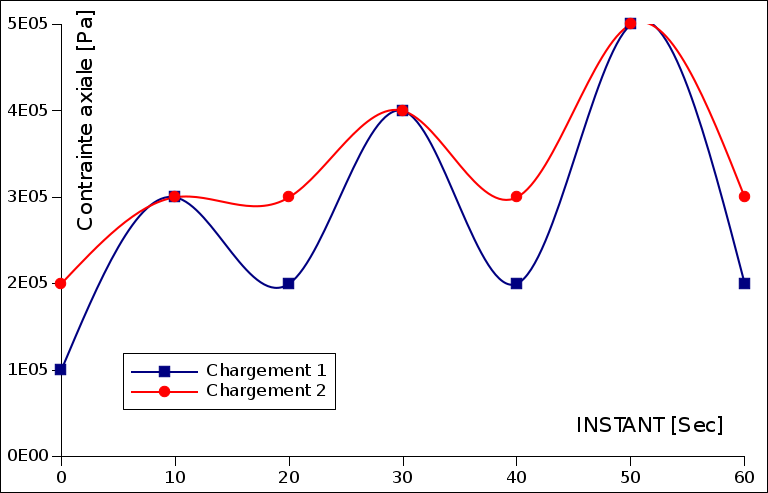
Figure 3.10.4-a : Oedometric loadings

For this example, the table below shows the simulation results contained in tables TABRES1 and TABRES2, as well as the order in which these tables are filled.

SIGM_IMPOSE		3.E5	4.E5	5.E5
PRES_CONF	SIGM_DECH	3.E5	4.E5	5.E5
1.E5	2.E5	TABRES1	TABRES1	TABRES1
2.E5	3.E5	TABRES2	TABRES2	TABRES2

Below is an extract from table TABRES2 containing the raw results of the simulations run for the second value of PRES_CONF, and SIGM_DECH

#——————————————————————————–

# ESSAI_OEDO_C number 1/PRES_CONF = -2.000000E+05/SIGM_DECH = -3.000000E+05

SIGM_IMPOSE_2 INST_2 EPS_VOL_2 P_2 SIG_AXI_2 SIG_LAT_2

-3.00000E+05 0.00000E+00 0.00000E+00 -2.00000E+05 -2.00000E+05 -2.00000E+05 -2.00000E+05

-3.00000E+05 4.00000E-01 -7.39723E-05 -2.01077E+05 -2.12000E+05 -1.95616E+05

-3.00000E+05 8.00000E-01 -1.75678E-01 -1.75678E-04 -2.02549E+05 -2.24000E+05 -1.91824E+05

-3.00000E+05 1.20000E+00 -3.18644E-04 -2.04590E+05 -2.36000E+05 -1.88885E+05 -1.88885E+05

-3.00000E+05 1.60000E+00 -4.99908E-04 -2.07143E+05 -2.48000E+05 -1.86714E+05

-3.00000E+05 2.00000E+00 -7.15464E-04 -2.10149E+05 -2.60000E+05 -1.85224E+05

-3.00000E+05 2.40000E+00 -9.61164E-04 -2.13554E+05 -2.72000E+05 -1.84332E+05 -1.84332E+05

-3.00000E+05 2.80000E+00 -1.23276E-03 -2.17306E+05 -2.84000E+05 -1.83959E+05

-3.00000E+05 3.20000E+00 -1.52656E-03 -2.21361E+05 -2.96000E+05 -1.84041E+05

-3.00000E+05 3.60000E+00 -1.83869E-03 -2.25674E+05 -3.08000E+05 -1.84511E+05 -1.84511E+05

-3.00000E+05 4.00000E+00 -2.16608E-03 -2.30211E+05 -3.20000E+05 -1.85317E+05 -1.85317E+05

-3.00000E+05 2.00000E+01 -6.04300E-03 -2.76465E+05 -3.00000E+05 -2.64698E+05 -2.64698E+05

-4.00000E+05 2.04000E+01 -6.11132E-03 -2.80404E+05 -3.16000E+05 -2.62606E+05 -2.62606E+05

-4.00000E+05 2.08000E+01 -6.19529E-03 -2.81924E+05 -3.32000E+05 -2.56886E+05 -2.56886E+05

-4.00000E+05 2.12000E+01 -6.28651E-03 -2.83575E+05 -3.48000E+05 -2.51363E+05

-4.00000E+05 2.16000E+01 -6.39457E-03 -2.85529E+05 -3.64000E+05 -2.46293E+05 -2.46293E+05

-4.00000E+05 2.20000E+01 -6.51836E-03 -2.87762E+05 -3.80000E+05 -2.41643E+05

-4.00000E+05 2.24000E+01 -6.65666E-03 -2.90254E+05 -3.96000E+05 -2.37381E+05 -2.37381E+05

-4.00000E+05 2.28000E+01 -6.80833E+01 -6.80833E-03 -2.92984E+05 -4.12000E+05 -2.33476E+05

-4.00000E+05 2.32000E+01 -6.97209E+01 -6.97209E-03 -2.95933E+05 -4.28000E+05 -2.29900E+05

-4.00000E+05 3.96000E+01 -1.01176E-02 -3.27727E+05 -3.16000E+05 -3.33591E+05

-4.00000E+05 4.00000E+01 -9.76282E+01 -9.76282E-03 -3.20137E+05 -3.00000E+05 -3.30206E+05

-5.00000E+05 4.04000E+01 -9.84598E-03 -3.24672E+05 -3.20000E+05 -3.04000E+05 -3.27007E+05

-5.00000E+05 4.08000E+01 -9.94584E-03 -3.26579E+05 -3.40000E+05 -3.19868E+05 -3.19868E+05

-5.00000E+05 4.12000E+01 -1.00631E-02 -3.28816E+05 -3.60000E+05 -3.12000E+05 -3.13225E+05

-5.00000E+05 4.16000E+01 -1.02034E-02 -3.31485E+05 -3.80000E+05 -3.07228E+05 -3.07228E+05

3.10.5. Operand GRAPHIQUE, PREFIXE_FICHIER#

◊ GRAPH = | ('P-EPS_VOL', 'SIG_AXI-EPS_VOL') [DEFAULT]

| l_graph [l_KN]

◊ PREFIXE_FICHIER = prefix [Kn]

Same as in § 3.4.5.

3.10.6. Operand NOM_CMP#

◊ NOM_CMP = l_component [L_kn]

Same as in § 3.4.6.

3.10.7. Operand TABLE_REF#

◊ TABLE_REF = l_tabref [l_table]

Same as in § 3.4.7.

3.10.8. Operands COULEUR, MARQUEUR, STYLE#

◊ COULEUR = l_color [L_i]

◊ MARQUEUR = l_marker [L_i]

◊ STYLE = l_style [L_i]

Same as in § 3.4.8.

3.11. Keyword ESSAI_ISOT_DR_C#

This keyword factor (repeatable) makes it possible to perform a series of simulations of the same cyclic drained isotropic compression test for which the loading parameters are varied (initial isotropic consolidation pressure, magnitude of isotropic effective stress imposed, and magnitude of isotropic discharge stress), to post-process the results obtained and to write them in the form of graphs (in xmgrace format) and/or tables.

3.11.1. Entry and exit sign agreement#

Same as in § 3.10.1.

3.11.2. Operands PRES_CONF, SIGM_IMPOSE, SIGM_DECH, NB_CYCLE,, NB_INST, TYPE_CHARGE#

♦ PRES_CONF = l_sigma_conf [L_r]

♦ SIGM_IMPOSE = l_sigma_impo [L_r]

♦ SIGM_DECH = l_sigma_discharge [L_r]

♦ NB_CYCLE = nbcyc [I]

◊ NB_INST = | 25 [DEFAULT]

| nbinst [I]

◊ CHARGE_TYPE = | 'SINUSOIDAL' [DEFAULT]

|'TRIANGULAR' [Kn]

Same as in § 3.10.2 with \({K}_{0}=1\).

3.11.3. Operand TABLE_RESU#

◊ TABLE_RESU = l_tabres [L_co]

Same as in § 3.10.4.

3.11.4. Operand GRAPHIQUE, PREFIXE_FICHIER#

◊ CHART = |'P-EPS_VOLL' [DEFAULT]

| l_graph [l_KN]

◊ PREFIXE_FICHIER = prefix [Kn]

Same as in § 3.4.5.

3.11.5. Operand NOM_CMP#

◊ NOM_CMP = l_component [L_kn]

Same as in § 3.4.6.

3.11.6. Operand TABLE_REF#

◊ TABLE_REF = l_tabref [l_table]

Same as in § 3.4.7.

3.11.7. Operands COULEUR, MARQUEUR, STYLE#

◊ COULEUR = l_color [L_i]

◊ MARQUEUR = l_marker [L_i]

◊ STYLE = l_style [L_i]

Same as in § 3.4.8.