3. Operands#
3.1. Modal basis of the structure#
3.1.1. Operand MODE_MECA#
♦ MODE_MECA = fashion
The name of the mode_meca concept produced by the modal analysis operator CALC_MODES [U4.52.02].
3.1.2. Operands TOUT_ORDRE/NUME_ORDRE/NUME_MODE/LIST_ORDRE#
/TOUT_ORDRE = 'OUI'
Value by default that allows you to extract all the specific modes available in the concept mode.
/NUME_ORDRE = l_order

/NUME_MODE = l_mode
Extraction of the specific modes defined by a list l_order of order numbers (NUME_ORDRE) or a list l_mode of mode numbers (NUME_MODE).
/LIST_ORDRE = l_order
Same as NUME_ORDRE but of the listis type (produced by DEFI_LIST_ENTI).
3.1.3. Operand FREQ/LIST_FREQ/PRECISION/CRITERE#
/FREQ = l_freq
Allows you to extract the natural modes corresponding to a list of frequencies l_freq.
/LIST_FREQ = lfreqr8
Allows you to extract the natural modes corresponding to a list of frequencies lfreqr8, defined by the operator DEFI_LIST_REEL [U4.34.01] (lfreqr8 is therefore a listr8 concept).
I CRITERE =
These operands make it possible to indicate that we are looking for all the natural modes whose frequency is in the interval \(\mathit{inst}\mathrm{\pm }\mathit{prec}\). By default \(\mathit{prec}\mathrm{=}\mathrm{1.0D}\mathrm{-}3\).
Based on the value of the CRITERE keyword:
“RELATIF”: the search interval is:
“ABSOLU”: the search interval is:
3.2. Modal amortization#
Three possibilities exist to define modal amortizations: a list of reduced depreciations provided by the user in the form of a list of reals (L_r) or a listr8 concept constructed by the operator DEFI_LIST_REEL [U4.34.01] or a generalized depreciation matrix (depreciation matrix projected on the basis of real eigenmodes).
3.2.1. Operand AMOR_REDUIT#
/AMOR_REDUIT = love
This operand makes it possible to provide the list of reduced amortizations in the form of a list of reals (L_r). If the number of coefficients provided is less than the number of natural modes taken into account, the last coefficient is assigned to the corresponding mode and to the following modes.
3.2.2. Operand LIST_AMOR#
/LIST_AMOR = lamor
This operand makes it possible to provide the list of reduced depreciations in the form of a listr8 concept. If the number of reduced depreciations is less than the number of natural modes taken into account, the last coefficient is assigned to the following modes.
Example:
LIST_AMOR =( “0.01”, “0.02”)
first mode \(\xi \mathrm{=}\text{0.01}\) and for all other modes \(\xi =\text{0.02}\)
3.2.3. Operand AMOR_GENE#
/AMOR_GENE = amogenous
The name of the amogenous generalized damping matrix produced by the operator PROJ_MATR_BASE [U4.63.12] or PROJ_BASE [U4.63.11] is given.
Note:
For theoretical reasons (framework of COMB_SISM_MODALrestreint to « classical » damping) the damping matrix must be **diagonal.*
3.3. Pseudo-mode corrections: operand MODE_CORR#
The modal base used is generally incomplete. The evaluation of the probable mean magnitude of the response to seismic excitation therefore requires a correction by a term representing the contribution of the neglected natural modes, in each earthquake direction, called pseudo-mode correction or static correction.
For each direction of the earthquake, this correction is carried out by adding to the modal base, a pseudo‑mode \(\Psi\) obtained from a static mode \(\varphi\), the field of movement of the nodes of the structure subjected to uniform acceleration in the direction considered defined by:
\(K\varphi =M\delta\)
\(K\) structural stiffness matrix
\(M\) mass matrix of the structure
\(\delta\) unit field in the direction of the earthquake
The pseudo-mode \(\Psi\) is obtained by subtracting the static contributions of the modes taken into account:
\(\Psi =\varphi -\sum _{r=1}^{\mathrm{nmod}}\frac{{p}_{r}}{{\omega }_{r}^{2}}{\Phi }_{r}\)
with:
\({\Phi }_{r}\) clean index \(r\) mode
\({p}_{r}\) management participation factor \(\delta\)
In this direction \(\delta\), for each quantity, the contribution of the neglected modes is given by:
\({R}_{t}={R}_{s}-\sum _{r=1}^{\mathrm{nmod}}{R}_{r}\)
\({R}_{s}\) is the quantity associated with static mode
The definition of pseudo-mode correction is as follows:
◊ MODE_CORR =/”OUI”
◊ FREQ_COUP = freq [R] /”NON” [DEFAUT]
Only if MODE_CORR = 'OUI':


♦ PSEUDO_MODE = access
Mandatory if MODE_CORR = “OUI”, this keyword makes it possible to provide the field (s) for movements \(\phi\) of the nodes of the structure subjected to uniform acceleration in one (or more) direction (s), field (s) calculated by the operator MODE_STATIQUE with the keyword PSEUDO_MODE [U4.52.14]. For specific needs, it is also possible to provide a concept from CREA_RESU, by choosing TYPE_RESU =” MODE_MECA “and entering the keyword AXE of AFFE to indicate the direction corresponding to each field (defined by its order number) [U4.44.12]. For any earthquake direction where the response is calculated, a pseudo-mode is calculated if access is provided.
For other quantities of interest (see options § 3.7) other than displacement, it is important to calculate these quantities mode by mode via CALC_CHAMP using the travel fields \(\varphi\) from the travel fields from the operator MODE_STATIQUE/PSEUDO_MODE.
In principle, the static calculation of the displacement fields \(\phi\) at the nodes of the structure subjected to uniform acceleration via MODE_STATIQUE/PSEUDO_MODE, it is therefore impossible to deduce from them the fields of the responses in relative speed or in absolute acceleration. Thus, it is impossible to take into account the static correction by pseudo-mode for the options” VITE “,” ACCE_ABSOLU “(see the options § 3.7) with the exception of the absolute acceleration response in the case of mono-support where we know analytically the absolute acceleration field” ACCE_ABSOLU “of the structure subjected to uniform acceleration. This is the unit field of absolute acceleration at ddls in translations. This correction is automatically performed regardless of the entry of the MODE_CORR keyword.
This keyword makes it possible to provide the frequency with which we read on the SRO the value that will be used for the correction level by pseudo-mode. This frequency normally corresponds to the cutoff frequency of the seismic signal, i.e. the one where SRO reaches (in absolute pseudo-acceleration) an asymptote. This keyword is particularly useful when the last frequency of the modal base does not reach the cutoff frequency of the seismic signal although it is nevertheless sufficient to take into account all the predominant modes for the response of the structure (practice not recommended).
The value entered in FREQ_COUP is applied for all earthquake directions taken into account in the analysis.
In case of absence of this keyword, the last existing frequency in the modal base MODE_MECA is used as soon as the pseudo-mode correction is activated (MODE_CORR = “OUI”). In addition, the spectral value read from the spectrum corresponds to the lowest damping value.
3.4. Excitation type (single-press or multi-press)#
Two configurations are possible:
mono-support: the structure is designed with the same driving movement at all supports
multi-support: the structure is studied with several different drive movements at the supports and possibly differential movements of the supports (DDS)
The treatment of the two types of arousal is different. The type of analysis is adequately defined by the user via the TYPE_ANALYSE operand
♦ TYPE_ANALYSE =/”MONO_APPUI” [DEFAUT]
/”MULT_APPUI”
3.5. Loading description#
Seismic loading is defined by:
one or more oscillator spectra
differential movements of the support only in case of multi-support
3.5.1. Mono-support#
Only oscillator spectra are defined for the case of mono-support.
♦ SPECTRE =_F (♦ LIST_AXE = l_axis] [l_axis]
◊ ECHELLE = scale [R] ◊ CORR_FREQ =/”OUI” /”NON” [DEFAUT] ◊ NATURE =/”ACCE” [DEFAUT] /”VITE” /”DEPL” )
3.5.1.1. Oscillator spectrum#
♦ SPEC_OSCI = specification
A single sheet of oscillator spectra where spec is the name of the sheet to use (oscillator spectra parameterized by the value of the reduced damping). This spectrum is calculated beforehand by the command CALC_FONCTION [U4.32.04] or read from a file by the command LIRE_FONCTION [U4.32.02]. In both cases, the product concept is a function with two variables (tablecloth).
◊ ECHELLE = ladder
An echel scale factor to be applied at all points in the spec. spectrum.
Size of the oscillator spectrum. By default, we use an absolute pseudo-acceleration spectrum “ACCE”. It is possible to use other quantities more rarely: speed “VITE” (relative pseudo-speed) or displacement “DEPL” (relative displacement).
♦ LIST_AXE = (
“X”,“Y”,“Z”,)
At each occurrence of the keyword factor, the axes concerned by the excitation described via a list composed of “X”, “Y” and “Z” are specified.
◊ CORR_FREQ =/'OUI'
/”NON” [DEFAUT]
In fact, to calculate the displacement response components from an oscillator spectrum in pseudo-absolute acceleration (NATURE = “ACCE”) or pseudo-relative speed (NATURE = “VITE”), one has to divide each value twice or once by \({\omega }_{r}\) pulsation of the real eigenmode (undamped oscillator). In all seriousness the oscillator \(r\) is damped and its natural pulsation is \({\omega }_{r}\sqrt{1-{\xi }^{2}}\) and \({\omega }_{r}\) is only the proper pseudo-pulsation. The operand CORR_FREQ = “OUI” allows you to correct these values to take into account the damping of the eigenmode:
\(\begin{array}{ccccc}{\mathit{vite}}_{\mathit{max}}& \text{=}& {\omega }_{r}\sqrt{1-{\xi }^{2}}{\mathit{depl}}_{\mathit{lu}}& \text{=}& \mathit{vitesse}\hfill \\ {\mathit{acce}}_{\mathit{max}}& \text{=}& {\omega }_{r}^{2}\left(1-{\xi }^{2}\right){\mathit{depl}}_{\mathit{lu}}& \text{=}& \mathit{accélération}\hfill \end{array}\)
If a response spectrum is provided in relative pseudo-speed (NATURE = “VITE”), the operand CORR_FREQ will be necessary to correct \({\mathrm{depl}}_{\mathrm{max}}\) and \({\mathrm{acce}}_{\mathrm{max}}\) if necessary. Likewise for an absolute pseudo-acceleration response spectrum (NATURE = “ACCE”) to correct \({\mathit{depl}}_{\mathit{max}}\) and \({\mathit{vite}}_{\mathit{max}}\).
Example:
For a ground spectrum with absolute pseudo-acceleration sol_0_1 set to \(0.1m/{s}^{2}\) and a scale factor making it possible to simulate a spectrum set to \(0.25m/{s}^{2}\), applied to three global directions, and without taking into account the correction of the frequencies:
♦ SPECTRE =_F (SPEC_OSCI =sol_0_1,
NATURE =” ACCE “, LIST_AXE =( “X”, “Y”, “Z”,),
CORR_FREQ = “NON”,
)
3.5.2. Multi-support#
In the case of multi-support, the structure is studied with several different movements at the supports. There are two configurations:
Multi-support correlated: all supports are correlated with each other;
Uncorrelated multi-support: we can show groups that are perfectly uncorrelated with each other, the excitations within the same support group being assumed to be correlated with each other.
Thus, the steps for defining the load are as follows:
Definition of supports via operand APPUIS
Definition of correlated support groups via operand GROUP_APPUI_CORRELE
Definition of oscillator spectra (SRO) for each press via the SPECTRE operand
Definition of Differential Seismic Displacements (DDS) for each support via the DEPL_MULT_APPUI operand
3.5.2.1. Operand APPUIS#
♦ APPUIS =_F (♦ NOM = support_name
where:
♦ NOM = support_name
Character string (limited to 4 characters maximum) defined by the user to designate the name of the support.
3.5.2.3. Operand SPECTRE#
The spectra are defined for each support via the factor SPECTRE as the case for the mono-support with, in addition:
♦ NOM_APPUI = support_name: the name of the support concerned
3.5.2.4. Operand DEPL_MULT_APPUI#
Since the training movement of the structure is not uniform, this keyword makes it possible to define the contribution to the overall response of a list of supports or support groups. This is established on the basis of the static modes with imposed movements of the structure:
\({R}_{\mathrm{ei}}={\Phi }_{\mathrm{si}}{\delta }_{i\mathrm{max}}\)
with:
\({\Phi }_{\mathrm{si}}\) |
static mode for \(i\) support |
\({\delta }_{i\mathrm{max}}\) |
maximum displacement of the \(i\) support in relation to a reference support (for which \({\delta }_{i\mathit{max}}\mathrm{=}0\)) |
If this keyword is not specified, then the contribution of the static modes of the structure is zero. In other words, this is equivalent to entering \({\delta }_{i\mathrm{max}}=0\).
DDS are defined by occurrences of the DEPL_MULT_APPUI factor:
◊ DEPL_MULT_APPUI =_F (♦ NOM_APPUI = support_name
◊ GROUP_NO_REFE = lgrno [l_gr_node]
♦ GROUP_NO = lgrno [l_gr_node] ♦ | DX = DX [R] | DY = dy [R] | DZ = dz [R]
)
♦ NOM_APPUI = support_name
Name of the support concerned
Static mode name \({\Phi }_{\mathit{si}}\), mode_stat type concept produced by the MODE_STATIQUE operator, keyword MODE_STAT [U4.52.14].
Group containing the reference node in relation to which the relative movements of the supports are defined (the given group must contain only one node).
If this operand is present, the maximum displacement applied to support \(i\) is equal to \({\delta }_{i\mathit{max}}\mathrm{-}\Delta\) where \(\Delta\) is the displacement assigned to the reference node node in the direction in question.
List of the names of the groups of nodes corresponding to the supports concerned by the occurrence of the keyword factor DEPL_MULT_APPUI.
I DY= dy I DZ= DZ
Maximum relative displacement value of the supports concerned, direction by direction.
In principle, the static calculation of the displacement fields \(\phi\) at the nodes of the structure subjected to a displacement imposed on a given support via MODE_STATIQUE, it is impossible to deduce from them the fields the responses in relative speed or in absolute acceleration. Thus, it is impossible to take into account DDS for the options” VITE “,” ACCE_ABSOLU “(see options § 3.7).
Example:
A pipe line is fixed to two distinct floors via different supports. Two supports (sup1 and sup2) are located on the level 1 floor, while (sup3 and sup4) are located on the level 2 floor. Four different spectra are defined. The movements of floor 1 and 2 are considered to be decorrelated, while all spectra on the same floor are considered to be correlated.
_F (NOM = »sup1 », GROUP_NO = » NO1 « ), _F (NOM = »sup2 », GROUP_NO = » NO2 « ), _F (NOM = »sup3 », GROUP_NO = » NO3 « ), _F (NOM = »sup4 », GROUP_NO = » NO4 « ),
),
GROUP_APPUI_CORRELE =(
_F (LIST_APPUI =( « sup1 », « sup2 »,), NOM = »plank_1 »),
_F (LIST_APPUI =( « sup3 », « sup4 »,), NOM = »plank_2 »),
),
SPECTRE =(
_F (NOM_APPUI = »sup1 », LIST_AXE =( « X »), SPEC_OSCI = SRO1_NO1,),
_F (NOM_APPUI = »sup2 », LIST_AXE =( « X »), SPEC_OSCI = SRO1_NO2,),
_F (NOM_APPUI = »sup3 », LIST_AXE =( « X »), SPEC_OSCI = SRO2_NO1,),
_F (NOM_APPUI = »sup4 », LIST_AXE =( « X »), SPEC_OSCI = SRO2_NO2,),
),
DEPL_MULT_APPUI =(
_F (MODE_STAT = MODE_STA, NOM_APPUI = »sup1 », DX= DDS1),
_F (MODE_STAT = MODE_STA, NOM_APPUI = »sup2 », DX= DDS2),
_F (MODE_STAT = MODE_STA, NOM_APPUI = »sup3 », DX= DDS3),
_F (MODE_STAT = MODE_STA, NOM_APPUI = »sup4 », DX= DDS4),
),
3.6. Combination rules#
We reason quantity by quantity (displacement, speed or acceleration, internal forces, constraints) from the modal values associated with the natural modes taken into consideration. For each quantity, each degree of freedom (fields at the nodes of movement, speed or acceleration), or each component of torsor (internal forces) or stress will be treated independently. This is what we call answer \(R\) in the combination rules statement.
Several levels of combinations are required:
combination of clean modes,
static correction by pseudo-mode,
combination according to earthquake directions.
In the case of a multi-support analysis, the combination rules are modified to take into account the various excitations applied to support groups. It is also possible to calculate the components of the inertial response and due to DDS separately.
3.6.1. Mono-support#
The calculation of the total response resulting from the accumulation of modal and then directional responses is shown in the figure.
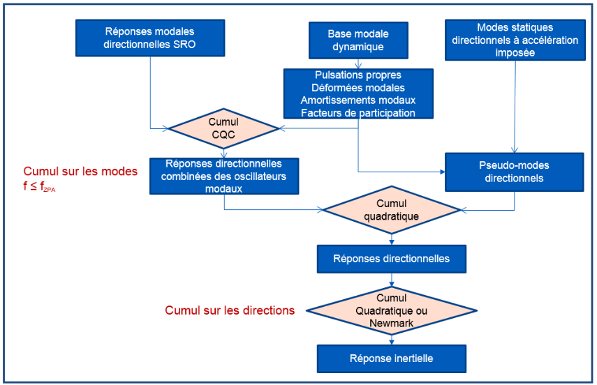
Figure 3.6.1-1: Single-support spectral calculation (Ref. [6])
The total response of the structure \(R\) is obtained by combining the directional answers \({R}_{X}\) where \(X\) represents one of the directions of the coordinate system GLOBAL defining the mesh \((X,Y,Z)\). The directional response is given by:
\({R}_{X}=\sqrt{{R}_{d}^{2}+{({R}_{t}+{R}_{\mathit{qs}})}^{2}}\)
\({R}_{d}\) dynamic combined response of modal oscillators established by the accumulation of modes with the rule defined by the keyword COMB_MODE [§ 3.6.3]
\({R}_{t}\) fix the static effects of overlooked modes (pseudo-mode) [§ 3.5.1.1]
\({R}_{\mathit{qs}}\) combined quasistatic answer of the modal oscillators established by the accumulation of modes only with the rule GUPTA “by the keyword COMB_MODE (TYPE =” GUPTA”) [§ 3.6.3.6]
The rule for combining directional responses is defined by the keyword COMB_DIRECTION [§ 3.6.4].
In summary, for the case of mono-support, the rule of the accumulation of modes is defined by the keyword COMB_MODE [§ 3.6.3] and directions by the keyword COMB_DIRECTION [§ 3.6.4].
3.6.2. Multi-support#
For the total response of the multi-support case, the sequence of accumulations is shown in the figure.
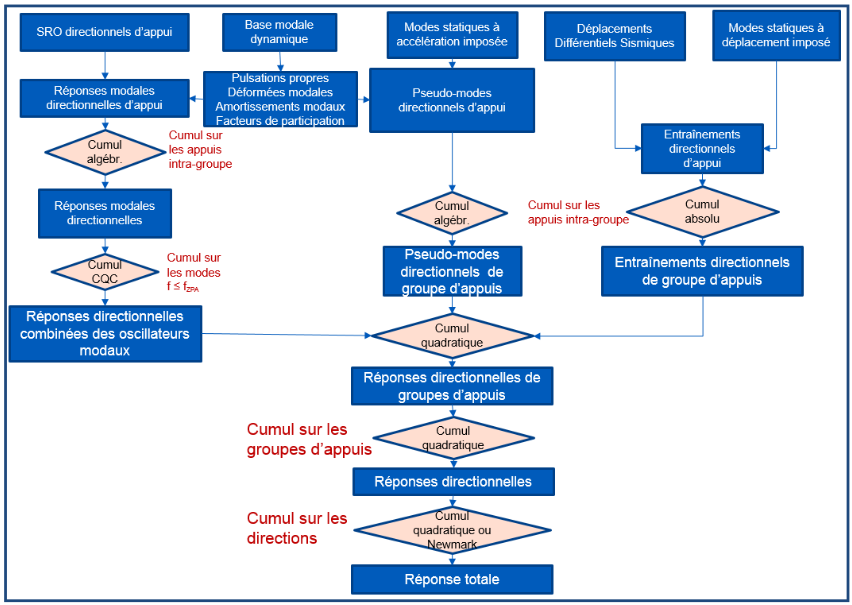
Figure 3.6.2-1: Multi-support spectral calculation (Ref. [6])
The total response of the structure \(R\) is obtained by combining the directional answers \({R}_{X}\) where \(X\) represents one of the directions of the coordinate system GLOBAL defining the mesh \((X,Y,Z)\). The directional response is given by:
\({R}_{X}=\sqrt{{R}_{d}^{2}+{R}_{t}^{2}+{R}_{e}^{2}}\)
\({R}_{d}\) dynamic combined response of modal oscillators established by the accumulation of modes with the rule defined by the keyword COMB_MODE [§ 3.6.3]
\({R}_{t}\) fix the static effects of overlooked modes (pseudo-mode) [§ 3.3]
\({R}_{e}\) response to the training movement [§ 3.5.2.4]
For the combined dynamic response \({R}_{d}\) by direction, the combined dynamic responses of the various groups of correlated supports are cumulated quadratically (no choice left to the user for this inter-group accumulation):
\({R}_{d}=\sqrt{\sum _{m=1}^{\mathit{nbG}}{R}_{d,m}^{2}}\)
\({R}_{d,m}\) dynamic combined response of the modal oscillators for the m-th group of correlated supports
\(\mathit{nbG}\) total number of correlated support groups
For the dynamic response combined with the m-th support group \({R}_{d,m}\), we combine responses from the modes of the m-th support group correlated with the combination rule defined by the keyword COMB_MODE [§ 3.6.3] (example of illustration for the rule SRSS):
\({R}_{d,m}=\sqrt{\sum _{i=1}^{\mathit{nbM}}{R}_{d,m,i}^{2}}\)
\({R}_{d,m,i}\) dynamic combined response of the i-th mode for the m-th group of correlated supports
\(\mathit{nbM}\) total number of modes
For the dynamic response combined with the i-th mode to the m-th support group \({R}_{d,m,i}\), responses from the i-th mode of the correlated supports are accumulated linearly in the m-th correlated support group (no choice left to the user for this intra-group accumulation):
\({R}_{d,m,i}=\sum _{n=1}^{{\mathit{nbA}}_{m}}{R}_{d,m,i,n}\)
\({R}_{d,m,i,n}\) dynamic response from the i-th mode to SRO to the n-th press in the m-th correlated support group
\({\mathit{nbA}}_{m}\) total number of correlated supports constituting the m-th group of correlated supports
In summary, the combined dynamic response \({R}_{d}\) of the direction in question results from the linear accumulations of the correlated supports, and then, the accumulation of the modes by the rule defined by the keyword COMB_MODE [§ 3.6.3] and finally the quadratic accumulations of the support groups.
For the correction of the static effects of the neglected modes (pseudo-mode) combined \({R}_{t}\) by direction, we accumulate linearly corrections of the correlated supports in a group of supports and then quadratically the corrections of the groups of supports (no choice left to the user for these accumulations):
\({R}_{t}=\sqrt{\sum _{m=1}^{\mathit{nbG}}{R}_{t,m}^{2}}\)
\({R}_{t,m}=\sum _{m=1}^{{\mathit{nbA}}_{m}}{R}_{t,m,n}\)
\({R}_{t,m,n}\) correction due to SRO on the n-th press in the m-th correlated support group
\({\mathit{nbA}}_{m}\) total number of correlated supports constituting the m-th group of correlated supports
\({R}_{t,m}\) correction of the m-th correlated support group
\(\mathit{nbG}\) total number of correlated support groups
For the response to the training movement \({R}_{e}\) by direction, responses from correlated supports in a group of supports are accumulated in a group of supports by the rule defined in COMB_DDS_CORRELE (§ 3.6.5) and then quadratically responses from groups of supports (no choice left to the user for this inter-group accumulation). For this component, the rule for combining the DDS of the correlated supports is in absolute value, by default (illustration formula with absolute rule):
\({R}_{e}=\sqrt{\sum _{m=1}^{\mathit{nbG}}{R}_{e,m}^{2}}\)
- math:
{R} _ {e, m} =sum _ {m=1} ^ {{mathit {nBa}} _ {m}}left| {R} _ {e} _ {e, m, n}right|
\({R}_{e,m,n}\) response due to DDS at the n-th press in the m-th correlated support group
\({\mathit{nbA}}_{m}\) total number of correlated supports constituting the m-th group of correlated supports
\({R}_{e,m}\) combined response from the m-th correlated support group
\(\mathit{nbG}\) total number of correlated support groups
In summary, for the case of multi-support, the first accumulation being linear is carried out between the various nodes (NOEUD) of the same support for all the components without a choice left to the user. Next, the rule of intra-group accumulation (responses between correlated supports within the same group) is linear for the responses of the oscillators and the pseudo-mode (no user choice) while for the answer to DDS, the rule is defined in COMB_DDS_CORRELE (§ 3.6.5). Next, the accumulation of modes is defined by the keyword COMB_MODE [§ 3.6.3], then, the quadratic accumulation of support groups (quadratic inter-group accumulation without user choice). Finally, the accumulation of directions is defined by the keyword COMB_DIRECTION [§ 3.6.4].
3.6.3. Combining clean modes: keyword COMB_MODE#
The response of the structure \({R}_{d}\), in an earthquake direction, is obtained by one of the possible combinations (defined by the TYPE operand) of the contributions of each of the natural modes taken into account. Each eigenmode is considered to be an independent oscillator with response \({R}_{r}\) defined by \(({\omega }_{r},{\xi }_{r})\). The response is read by interpolation in the oscillator spectrum of the excitation signal in this direction.
For single-press excitation, the \({R}_{r}\) response of the \(r\) oscillator is given by:
\({R}_{r}=\frac{{p}_{r}}{{\omega }_{r}^{2}}{S}_{r}{\Phi }_{r}\)
|
modal quantity (displacement, generalized effort, reaction) associated with the natural mode with index \(r\) |
|
modal participation factor associated with the \(r\) mode in the direction studied |
|
value of the response spectrum, for example in pseudo-acceleration, for the \(r\) oscillator, for the specified damping value |
Several rules for combining specific modes are available. They are chosen by the operand TYPE. The rule for combining natural modes is common for all directions under consideration.
3.6.3.1. Quadratic combination TYPE = “SRSS”#
This combination (Square Root of Sum of Squares) corresponds to the hypothesis of strict independence of the oscillators associated with each specific mode:
\({R}_{d}=\sqrt{\sum _{r=1}^{\mathit{nmod}}{R}_{r}^{2}}\)
Note that this combination rule, although very commonly used, can be poorly adapted when the independence hypothesis is not verified for neighboring or highly damped eigenmodes.
3.6.3.2. Full quadratic combination TYPE = “CQC”#
The quadratic combination (established by DER KIUREGHIAN [bib1]) provides a correction to the previous rule by introducing correlation coefficients depending on damping and on the distances between neighboring eigenmodes (cf. [R4.05.03]):
\({R}_{d}=\sqrt{\sum _{{r}_{1}}\sum _{{r}_{2}}{\rho }_{{r}_{1}{r}_{2}}{R}_{{r}_{1}}{R}_{{r}_{2}}}\)
with the correlation coefficient:
\({\rho }_{\mathrm{ij}}=\frac{8\sqrt{{\xi }_{i}{\xi }_{j}{\omega }_{i}{\omega }_{j}}({\xi }_{i}{\omega }_{i}+{\xi }_{j}{\omega }_{j}){\omega }_{i}{\omega }_{j}}{{({\omega }_{i}^{2}-{\omega }_{j}^{2})}^{2}+4{\xi }_{i}{\xi }_{j}{\omega }_{i}{\omega }_{j}({\omega }_{i}^{2}+{\omega }_{j}^{2})+4({\xi }_{i}^{2}+{\xi }_{j}^{2}){\omega }_{i}^{2}{\omega }_{j}^{2}}\)
3.6.3.3. Sum of absolute values TYPE = “ABS”#
This combination corresponds to a hypothesis of complete dependence of the oscillators associated with each specific mode:
- math:
{R} _ {d} =sum _ {r=1} ^ {mathit {nmod}}left| {R} _ {r}right|
Note that this combination rule is not recommended, because it is too strongly conservative and leads to systematic oversizing.
3.6.3.4. Combination with 10% rule TYPE = “DPC”#
Neighboring modes (whose frequencies differ by less than 10%) are first combined by summing the absolute values. The values resulting from this first combination are then combined quadratically. This method was proposed by the American regulation U.S. Nuclear Regulatory Commission (Regulatory Guide 1.92 - February 1976) to mitigate the conservatism of the previous method. It is still lacking for structures with high modal density.
The \(i\) and \(i+1\) modes are similar when:
\(2\frac{({f}_{i+1}-{f}_{i})}{({f}_{i+1}+{f}_{i})}\le 10\text{\%}\)
3.6.3.5. Combination of ROSENBLUETH TYPE = “DSC”#
This rule (proposed by E. ROSENBLUETH and J. ELORDY [bib2]) introduces a correlation between modes, different from that of the CQC method. The responses of the oscillators are combined by double sum (Double Sum Combination):
\({R}_{d}=\sqrt{\sum _{{r}_{1}}\sum _{{r}_{2}}{\rho }_{{r}_{1}{r}_{2}}{R}_{{r}_{1}}{R}_{{r}_{2}}}\)
It requires additional data, the duration \(s\) of the « strong » phase of the earthquake defined by the operand DUREE. The user must ensure the homogenization of the units, the frequency is in Hz, so the duration must be in seconds.
The correlation coefficient is then:
\(\begin{array}{c}{\rho }_{\mathit{ij}}={\left(1+{\left(\frac{\omega {\text{'}}_{i}-\omega {\text{'}}_{j}}{\xi {\text{'}}_{i}{\omega }_{i}+\xi {\text{'}}_{j}{\omega }_{j}}\right)}^{2}\right)}^{-1}\\ \mathit{où}\phantom{\rule{2em}{0ex}}\omega {\text{'}}_{i}={\omega }_{i}\sqrt{1-{\xi }_{i}^{2}}\phantom{\rule{2em}{0ex}}\mathit{et}\phantom{\rule{2em}{0ex}}\xi {\text{'}}_{i}={\xi }_{i}+\frac{2}{s{\omega }_{i}}\end{array}\)
3.6.3.6. Gupta combination TYPE = “GUPTA”#
Gupta [NRC1.92], to take into account the correlations between modes due to the quasi-static part of the response, introduces the rigid response factor, which varies from 0 to 1 the correlation between the modal responses of intermediate frequencies between \({\mathit{FREQ}}_{1}\) and \({\mathit{FREQ}}_{2}\), two frequencies to be determined by the user.
Gupta breaks down each \({R}_{r}\) modal response into a dynamic part \({R}_{r}^{p}\) and a semi-static part \({R}_{r}^{\mathit{qs}}\): \({R}_{r}^{\mathit{qs}}={\alpha }_{r}{R}_{r}\) and \({R}_{r}^{p}=\sqrt{1-{\alpha }_{r}^{2}}{R}_{r}\)
Thus, for each \(r\) mode, we assign the rigid response factor \({\alpha }_{r}\) to the modal response \({R}_{r}\):
\({\alpha }_{r}=0\) for \(f\le {f}_{1}\) and \({\alpha }_{r}=1\) for \(f\ge {f}_{2}\)
\({\alpha }_{r}\) is estimated for frequency \({f}_{r}\) using the following formula:
\({\alpha }_{r}=\frac{\text{ln}{f}_{r}/{f}_{1}}{\text{ln}{f}_{2}/{f}_{1}}\)
The dynamic combined response of the modal oscillators is carried out according to the combination “CQC”:
\({R}_{d}=\sqrt{\sum _{{r}_{1}}\sum _{{r}_{2}}{\rho }_{{r}_{1}{r}_{2}}{R}_{{r}_{1}}^{p}{R}_{{r}_{2}}^{p}}\)
The combined quasistatic response of the modal oscillators is carried out according to an algebraic combination:
\({R}_{\mathit{qs}}=\sum _{r=1}^{\mathit{nmod}}{R}_{r}^{\mathit{qs}}\)
This combination according to GUPTA is only available in the single-support case.
3.6.4. Combination according to directions: keyword COMB_DIRECTION#
◊ COMB_DIRECTION =/”QUAD”
/”NEWMARK” [DEFAUT]
Two rules for combining directional responses are available.
This operand is not mandatory. If there is more than one direction entered in operand SPECTRE, the COMB_DIRECTION = NEWMARK rule is applied by default. If there is only one direction entered in operand SPECTRE, no directional combinations are performed.
3.6.4.1. Quadratic combination: COMB_DIRECTION = “QUAD”#
This combination corresponds to the assumption of strict independence of responses in each direction:
\(R=\sqrt{{R}_{X}^{2}+{R}_{Y}^{2}+{R}_{Z}^{2}}\)
3.6.4.2. Combination of NEWMARK: COMB_DIRECTION = “NEWMARK”#
For each of the directions \(i(X,Y,Z)\), the 8 values are calculated:
\({R}_{i}=\pm {R}_{X}\pm \mathrm{0,4}{R}_{Y}\pm \mathrm{0,4}{R}_{Z}\)
This leads, by circular permutation, to 24 (respectively 8 and 2) values if 3 (respectively 2 and 1) directional excitations are defined
\({R}_{\mathit{max}}=\mathit{max}({R}_{i})\)
3.6.5. Keyword COMB_DDS_CORRELE#
◊ COMB_DDS_CORRELE =/”ABS” [DEFAUT]
/”QUAD” /”LINE”
This keyword defines the rule for combining responses to the training movements of correlated supports.
3.6.5.1. Quadratic combination COMB_DDS_CORRELE = “QUAD”#
\({R}_{e}=\sqrt{\sum {R}_{\mathit{ej}}^{2}}\)
3.6.5.2. Linear combination COMB_DDS_CORRELE = “LINE”#
\({R}_{e}=\sum _{j=1}^{\mathit{nbA}}{R}_{\mathit{ej}}\)
3.6.5.3. Absolute value combination COMB_DDS_CORRELE = “ABS”#
- math:
{R} _ {e} =sum _ {j=1} ^ {mathit {nA}}left| {R} _ {mathit {ej}}}right|
3.7. Calculation option: operand OPTION#
♦ OPTION
List of modal quantities (calculation options) whose combined response we want to determine:
“DEPL” |
relative displacement |
“VITE” |
relative speed |
“ACCE_ABSOLU” |
absolute acceleration = relative acceleration + training acceleration |
“SIGM_ELNO” |
element-wise constraints at nodes |
“SIEF_ELGA” |
element-wise constraints at integration points |
“SIPO_ELNO” |
constraints in the beam section broken down into the contributions of each generalized effort |
“EFGE_ELNO”, “SIEF_ELNO” |
generalized efforts by elements at the nodes |
“EGRU_ELNO” [U4.74.01] |
generalized efforts by elements at the nodes in the user coordinate system |
“REAC_NODA” |
reactions to support |
“FORC_NODA” |
internal efforts |
Note:
To calculate the force options or constraints on a part of the model defined by groups of cells, it is possible to combine a calculation on the concept mode produced by the operator CALC_CHAMP.
3.8. Output result type: operand TYPE_RESU#
It is possible to output several results by the occurrence of the operand
♦ TYPE_RESU =_F (TYPE = /” VALE_XXX “,
…
),
Depending on the type of result defined by the keyword TYPE, several keywords may be required to filter the output results:
Modal response: TYPE = /” VALE_SPEC “
Total answer: TYPE = /” VALE_TOTA “
Directional response: TYPE = /” VALE_DIRE “
Only if COMB_DIRECTION = “QUAD”:
Dynamic response: TYPE = /” VALE_DYNA “
Quasi-static response: TYPE = /” VALE_QS “
Inertial response: TYPE = /” VALE_INER “
Response to DDS (multi-press only): TYPE = /” VALE_DDS “
3.8.1. Modal response TYPE = /” VALE_SPEC “#
In mono-press, you can output the answers by mode and by direction:
\({R}_{d,i,k}={r}_{i}{\lambda }_{i,k}\frac{\mathit{SA}({f}_{i},{\xi }_{i})}{{{\omega }_{i}}^{2}}\)
where:
\({r}_{i}\) modal response (eigenmode vector) of the i-th mode
\({\lambda }_{i,k}\) modal participation factor of the i-th mode in the \(k=X,Y,Z\) direction
\(\mathit{SA}({f}_{i},{\xi }_{i})\) value read on the SRO at frequency \({f}_{i}\) and at damping \({\xi }_{i}\)
In multi-press, you can output the answers by mode, by press and by direction:
\({R}_{d,i,n,k}={r}_{i}{\lambda }_{i,n,k}\frac{{\mathit{SA}}_{n}({f}_{i},{\xi }_{i})}{{{\omega }_{i}}^{2}}\)
where:
\({r}_{i}\) modal response (eigenmode vector) of the i-th mode
\({\lambda }_{i,n,k}\) modal participation factor from the i-th mode per movement to the n-th press in the \(k=X,Y,Z\) direction
\({\mathit{SA}}_{n}({f}_{i},{\xi }_{i})\) value read on the SRO of the movement at the n-th press at the frequency \({f}_{i}\) and at the damping \({\xi }_{i}\)
# If TYPE = “VALE_SPEC”
◊/TOUT_ORDRE = “OUI” [DEFAUT] /NUME_ORDRE = l_order [L_i] /LIST_ORDRE = the order [listis] /NUME_MODE = l_mode [L_i] //FREQ = l_freq [L_r] /LIST_FREQ = lfreqr8 listr8 ◊ PRECISION =/ 1.D-3 [DEFAUT] /prec [R] ◊ CRITERE =/”RELATIF” [DEFAUT] /”ABSOLU” # only if MULT_APPUI ♦/TOUT_APPUI = “OUI” [DEFAUT]
/LIST_APPUI = l_support
3.8.1.1. Operands TOUT_ORDRE/NUME_ORDRE/NUME_MODE/LIST_ORDRE#
/TOUT_ORDRE = 'OUI'
Value by default that allows you to extract the results for all calculated eigenmodes
/NUME_ORDRE = l_order

/NUME_MODE = l_mode

/LIST_ORDRE = l_order
See § 3.1.2
3.8.1.2. Operand FREQ/LIST_FREQ/PRECISION/CRITERE#
See § 3.1.3
3.8.1.3. Operand TOUT_APPUI/LIST_APPUI#
Only used for the multi-support case.
/TOUT_ORDRE = “OUI”
Value by default that allows you to extract the results of the modes due to the movement of all the supports.
/LIST_APPUI = l_support
List of the names of the supports, defined by the keyword APPUIS (see § 3.5.2.1) for which the results are extracted.
3.8.2. Total answer TYPE = “VALE_TOTA”#
It is possible to leave:
If COMB_DIRECTION = “QUAD” the total answer
If COMB_DIRECTION = “NEWMARK” the maximum total response and the 24 (resp. 8 and 2) combinations corresponding to 3 directions of excitation (resp. 2 and 1) (see § 3.6.4.2)
# If TYPE = “VALE_TOTA”
♦ NEWMARK = “OUI” [DEFAUT]
activates the writing of the 24 (resp. 8 and 2) combinations corresponding to 3 directions of excitation (resp. 2 and 1)
3.8.3. Directional response TYPE = “VALE_DIRE”#
It is possible to output the directional response (see § 3.6):
\({R}_{X}=\sqrt{{R}_{d}^{2}+{R}_{t}^{2}+{R}_{e}^{2}}\)
# If TYPE = “VALE_INER”, “VALE_DDS”:
♦ LIST_AXE = l_axis
List of the axes concerned by the excitation described via a list composed of “X”, “Y” and “Z”.
3.8.4. Partition of inertial components and due to DDS of the answer#
For the seismic analysis of pipes, the partition of the inertial components and at DDS of the response may be necessary in order to post-treatment RCC -M [bib3]. It is possible to output these components for each direction as well as their combination by the rule COMB_DIRECTION = “QUAD” (and only that).
# If TYPE = “VALE_INER”, “VALE_DDS”:
♦ LIST_AXE = l_axis
List of the axes concerned by the excitation described via a list composed of “X”, “Y” and “Z”.
3.8.4.1. Inertial component: TYPE = “VALE_INER”#
For direction \(X\), the directional inertial component is defined as follows:
\({R}_{I,X}=\sqrt{{R}_{d,X}^{2}+{R}_{t,X}^{2}}\)
\({R}_{d,X}\) combined modal response from modal oscillators for the \(X\) direction (see § 3.6)
\({R}_{t,X}\) contribution of static correction of neglected modes (pseudo-mode) (see § 3.6)
The inertial component is the result of the quadratic accumulation of the three directional inertial responses:
\({R}_{I,\mathit{tot}}=\sqrt{{R}_{I,X}^{2}+{R}_{I,Y}^{2}+{R}_{I,Z}^{2}}\)
3.8.4.2. Component due to DDS: TYPE = “VALE_DDS”#
This is the static response induced by the seismic differential movements of the anchors (driving movement), only in case of multi-support. For the case of mono-support, this component is considered to be zero.
For direction \(X\), the directional component of the response due to DDS is defined as presented in § 3.6.2.
The component due to DDS is the result of the quadratic accumulation of the three directions:
\({R}_{E,\mathit{tot}}=\sqrt{{R}_{e,X}^{2}+{R}_{e,Y}^{2}+{R}_{e,Z}^{2}}\)
It should be noted that the intra-group accumulation of responses to DDS is carried out according to the rule defined by the user via COMB_DDS_CORRELE (§ 3.6.5.3) while the inter-group accumulation is quadratic with no choice left to the user.
3.8.5. Partition of dynamic and quasistatic contributions#
It is possible to output these shares for each direction as well as their combination by the rule COMB_DIRECTION = “QUAD” (and only that).
# If TYPE = “VALE_DYNA”, “VALE_QS”:
♦ LIST_AXE = l_axis
List of the axes concerned by the excitation described via a list composed of “X”, “Y” and “Z”.
3.8.5.2. Quasi-static part: TYPE = “VALE_QS”#
For the \(X\) direction, the directional quasistatic part \({R}_{t,X}\) is defined as the contribution of the static correction of the neglected modes (pseudo-mode) (see § 3.6).
The quasistatic part is the result of the quadratic accumulation of the three directional quasistatic responses:
\({R}_{t,\mathit{tot}}=\sqrt{{R}_{t,X}^{2}+{R}_{t,Y}^{2}+{R}_{t,Z}^{2}}\)
3.9. Operand TITRE#
◊ TITRE = t
Title attached to the concept produced by this operator [U4.03.01].
3.10. Operand INFO#
◊ INFO
General information:
name of the modal base used,
number of eigenvectors selected,
modal combination rule chosen,
calculation options requested.
Information on the modal basis taken into consideration (only the modes taken into account are printed):
mode number
mode frequency
participation factor
participatory modal mass (MASSE MODALE EFFECTIVE)
percentage of the participatory modal mass (MASSE MODALE UN EFFECTIVE)
Information on the spectra and the values read on the spectra at each press, each mode and each direction:
nature of the arousal
values read on the spectra taken into account corrections by CORR_FREQ
Information on static correction by pseudo-mode at each press and each direction:
how often the ZPA value is read
ZPA values taken into account corrections by CORR_FREQ
Information on combination rules:
Combination of responses to DDS between correlated supports
Combination of directional responses
/2: |
same as 1 |