3. Operands#

3.1. Operand RESULTAT#

/RESULTAT = resu

Name of a result concept such as evol_elas, evol_noli, dyna_trans or mode_meca. This operand makes it possible to recover the displacement field (and speed and acceleration for a dynamic calculation).

The model and the material field, which are required for the calculation, are also extracted from the result data structure. The possible calculation options for each type of modeling are listed in the table below.

	Calculation of \(G\)	Calculation of \(K\)
D_ PLAN/C_ PLAN	CALC_G	CALC_K_G
AXIS	CALC_G	CALC_K_G
3D	CALC_G	CALC_K_G

Table 3.1: Availability, by modeling, of calculation options.

Notes on material properties:

The characteristics of the material, retrieved from the resu data structure, are as follows:

Young’s modulus E,
NU Poisson’s ratio,
thermal expansion coefficient ALPHA (for a thermo-mechanical problem),
elastic limit SY (for a non-linear elastic problem),
slope of the tensile curve D_ SIGM_EPSI (for a nonlinear elastic problem with linear isotropic work hardening).

For the calculation of energy return, these characteristics may depend on the geometry (option “CALC_G”) and on the temperature (option “CALC_G”). They must be independent of temperature for the calculation of stress intensity factors.

The SY and D_ SIGM_EPSI characteristics are only treated for a nonlinear elastic problem with Von Mises work hardening. The calculation of stress intensity coefficients is treated only in linear elasticity.

Note:

For the calculation of stress intensity factors (option “ CALC_K_G “), the characteristics must be defined on all materials, including on the edge elements, due to the calculation method [R7.02.05]. To ensure this, it is advisable to do a AFFE = _F (TOUT = “OUI”) in the command AFFE_MATERIAU [U4.43.03], even if it means using the overload rule afterwards.

The stress intensity factors obtained with option CALC_K_Gsont calculated by evaluating the bilinear form of G with a purely mechanical singular solution (asymptotic Westergaard solution). If a thermo-mechanical problem is solved, the singularity due to the thermal field is then not taken into account.

An indicator of the error due to this approximation can be obtained by evaluating the difference between Get G_ IRWIN. In practice, the quantity \(\frac{∣G-{G}_{\mathit{irwin}}∣}{∣G∣}\) is evaluated at any point at the bottom of the crack, and the arithmetic mean is then calculated. If this average exceeds 50%, it is then estimated that we are outside the scope of validity of the approach, and an alarm message is sent.

Bi-material problem:

1st case: We have a bi-material but the crack point is in a single material, cf. Figure 3.1-a. If it is ensured that the crown, defined between the lower radii R_ INF and the upper radius R_ and the upper radius R_ SUP, has elements of the same material as support, the calculation is possible regardless of the option chosen. Otherwise only option “CALC_G” is possible.

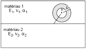
Figure 3.1-a: Bi-material: 1st case

2ndcas: We have a bi-material where the crack tip is at the interface, cf. Figure 3.1-b. To date, only the option for calculating the energy return rate (option “CALC_G”) is available. The calculation of stress intensity coefficients is not possible in this case.

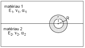
Figure 3.1-b: Bi-material: 2nd case

Calculation of equivalent stress intensity factors for a model with cohesive forces: For studies of crack propagation in the presence of cohesive forces, it may be necessary to calculate equivalent stress intensity factors, according to a very specific procedure of surface integrals on the cohesive zone, detailed in the reference documentation [R7.02.19]. Some syntax adjustments are then necessary:

the keywords R_ INF /R_ SUPne must not be entered, as it is not necessary to define a torus for field \(\theta\);
the COMPORTEMENTne keyword must not be entered, all information is extracted from the result;
only LAGRANGEet LAGRANGE_NO_NOsont smoothings available;
only option CALC_K_Gest available.

A typical syntax is provided at the end of this documentation.

3.2. Operands TOUT_ORDRE/NUME_ORDRE/LIST_ORDRE/INST//LIST_INST///TOUT_MODE/NUME_MODE//LIST_MODE/FREQ/purpose LIST_FREQ PRECISION CRITERE#

These operands are used with operand RESULTAT.

The operands TOUT_ORDRE, NUME_ORDRE, LIST_ORDRE, INST, LIST_INST are associated with evol_elas, evol_noli or dyna_trans results. See [U4.71.00].

The operands TOUT_MODE, NUME_MODE, LIST_MODE, FREQ, LIST_FREQ are associated with mode_meca results.

3.3. Keyword EXCIT and CHARGE/FONC_MULT operands#

◊ EXCIT = _F (♦ CHARGE = load

◊ FONC_MULT = fmult)

The keyword EXCIT makes it possible to retrieve a list of loaded loads, from commands AFFE_CHAR_MECA or AFFE_CHAR_MECA_F [U4.44.01], and the possible associated multiplier coefficients fmult.

The keyword EXCITest is optional and should not be entered in the general case.

If the EXCITest keyword is not present in the command, the load taken into account is the one extracted from resu. If the load is provided via EXCIT, then that load will be used in CALC_G_XFEM. If the load provided in EXCITest is different from that in resu (consistency of the name and number of charges, load-function pairs), an alarm is issued and the calculation continues with the loads indicated by the user. Attention, this use is only valid when the result is created via the CREA_RESU operator. Indeed, CREA_RESU allows you to define a result with or without applying loads. In the latter case, EXCITdonne has the ability to define the load directly in CALC_G_XFEM.

The loads currently supported by the various models and which may make sense in fracture mechanics are as follows:

Volume force: ROTATION, FORCE_INTERNE, PESANTEUR.
Surface force on the lips of the crack: FORCE_CONTOUR (2D), FORCE_FACE (3D), PRES_REP.
Thermal expansion: the temperature is transmitted via AFFE_MATERIAU/AFFE_VARC
In the event of a thermo-mechanical problem, the temperature is transmitted via the material properties (AFFE_MATERIAU/AFFE_VARC/EVOL). Thermal expansion is therefore automatically taken into account in the calculation with CALC_G.

Note:

Loads that are not supported by an option are **ignored. To date, the following loads that may make sense in fracture mechanics are not treated:*

FORCE_NODALE
FORCE_ARETE
DDL_IMPO on the lips of the crack
FACE_IMPO
PRE_EPSI

It is important to note that the only loads taken into account in a fracture mechanics calculation with method \(\theta\) are those supported by the elements inside the crown, where the vector field theta is non-zero (between R_ INF and R_ and R_ SUP [R7.02.01 §3.3]). The only types of load likely to influence the calculation of \(G\) **** are therefore the****volume loads (gravity, rotation), a non-uniform temperature field or forces applied to the lips of the crack. **

Attention:

If several loads of the same nature (for example, volume force) appear in the calculation, they are combined together for post-processing. However, it is currently not possible to make this combination if loads FORMULE are present: the calculation then ends in error. *
An exclusion rule is also applied when there is a simultaneous presence of a pre-deformation field (via “PRE_EPSI “) and an initial stress field.
It is not possible at this time to associate a load defined from a FORMULEet a multiplier coefficient ( FONC_MULT ). In this case, the calculation ends in error.
Kinematic loads ( AFFE_CHAR_CINE and AFFE_CHAR_CINE_F ) cannot be taken into account in the calculation.
For the option CALC_K_G , if a loading is imposed on the lips of the crack ( PRES_REP or FORCE_CONTOUR ), then it is required **obligatoryto orient their meshes correctly (using* ORIE_PEAU_2D or or*ORIE_PEAU_3D*) prior to calculating K (meshed crack case only) . *
If we do a calculation in large transformations (keyword DEFORMATION = “GROT_GDEP” or “PETIT_REAC”) the loads supported near the crack front (more exactly in the integration torus) must be dead loads, typically an imposed force and not a pressure [R7.02.03§2.4]; these loads must have been declared as non-follower in STAT_NON_LINE . However, follow-on loads can be defined far from the crack, because they are then not involved in the calculation of G.
Note that the calculation of CALC_G_XFEM with the modelling AXISn is not available for the results of thermo-mechanical calculations in large deformation and rotation.

3.4. Keyword THETA#

The theta field is calculated in CALC_G_XFEM using the keywords R_ INF /R_ INF_FO, R_ SUP /R_ SUP_FO and FISSURE.

The various cases are described in the table below according to the calculation option, the modeling (2D or 3D) and the type of crack (meshed crack or not).

	CALC_G	CALC_K_G
2D	◊ R_ INF, R_ SUP… ♦ FISSURE	◊ R_ INF, R_, R_ SUP… ♦ FISSURE
3D	◊ R_ INF, R_ SUP… ♦ FISSURE	◊ R_ INF, R_, R_ SUP… ♦ FISSURE

Tips on choosing crowns (in CALC_G_XFEM):

Avoid using a theta field defined with a lower radius R_ INF nil. The displacement fields are singular at the bottom of a crack and introduce inaccurate results in post-treatment of fracture mechanics.
It is recommended to use the command CALC_G_XFEM successively with at least three theta fields from different crowns to ensure the stability of the results. In case of significant variation (greater than 5-10%), it is necessary to question whether all the modeling is properly taken into account.
For the option CALC_K_Gen 2D-axisymmetric, the radius of the crowns must be small compared to the radius of the crack bottom to have the best possible precision. It is forbidden to have crowns with a radius greater than the radius of the crack bottom.

3.4.1. Operand FISSURE#

♦ FISSURE = kid,

This operand makes it possible to fill in the information relating to the crack defined by the DEFI_FISS_XFEM [U4.82.08] command.

This keyword is mandatory.

In the few cases where a propagation study is carried out with cohesive elements, this crack is of type COHESIF (keyword TYPE_DISCONTINUITE in DEFI_FISS_XFEM), and the operator then automatically calculates equivalent stress intensity factors by a specific method of surface integrals on the cohesive zone, detailed in [R7.02.19], §6.3.

3.4.2. Operands R_ INF, R_ INF_FO, R_, R_ SUP, R_ SUP_FO#

These operands make it possible to calculate the theta field when this one has not been previously determined. They correspond respectively to the lower and upper radii of the crowns (scalar or function, in 3D, of the curvilinear abscissa).

The two radii can be introduced either by constant real values that are arguments of simple keywords R_ INFet R_ SUP; or by functions of the curvilinear abscissa on the oriented crack background, which are arguments of the simple keywords R_ INF_FOet R_ SUP_FO.

Some tips are given below.

In 3D, when the radii are not a function of the curvilinear abscissa, the operands R_ INF and R_ SUP are optional. If they are not specified, they are automatically calculated from the maximum h of the mesh sizes connected to the nodes at the crack bottom. These mesh sizes at each bottom node are calculated in command DEFI_FISS_XFEM and are present in the concept or fiss_xfem [D4.10.01]. It was chosen to pose R_ SUP = 4h and R_ INF = 2h. If you choose the value automatically calculated for R_ SUP and R_ INF, you must however ensure that these values (displayed in the .mess file) are consistent with the dimensions of the structure.

In the case of a defect that is initially open and whose bottom is not flat, it is currently not possible to calculate the energy return rate.

3.4.3. Operand NUME_FOND#

◊ NUME_FOND = n,

This keyword is optional.

For some structures, it may happen that the crack bottom is discontinuous. In the case of a crack defined by DEFI_FISS_XFEM, the crack bottom is then cut into several parts.

The operand NUME_FOND makes it possible to indicate on which of these sub-parts of the crack bottom one wishes to perform the calculation. By default, the calculation is done on the first crack background.

3.4.4. Operand NB_POINT_FOND#

◊ NB_POINT_FOND = nbnofo,

This keyword is optional.

By default, the calculation is done on all the points of the crack background, that is to say all the points of intersection between the crack background and the edges of the mesh, for a non-meshed crack. The points at the bottom of the crack can be very irregularly spaced, which can lead to annoying oscillations on the calculated parameters \(G(s)\) or \(K(s)\).

The NB_POINT_FOND operand makes it possible to fix the number of post-processing points in advance, in order to improve the consistency of the results. The \(\mathit{nbnofo}\) points are evenly distributed along the crack bottom. Some tips are given in § 3.7.

This keyword can only be used for smoothing LAGRANGE - LAGRANGE.

3.5. Keyword COMPORTEMENT#

◊ COMPORTEMENT = _F (

This keyword factor makes it possible to redefine the behavior of the material. But the use of this keyword should not be systematic: in fact, by default, the law of behavior used in CALC_G_XFEM is identical to that used for mechanical calculation (via MECA_STATIQUE or STAT_NON_LINE). Entering the behavior keyword creates an Alarm, but the calculation continues, it is up to the user to verify that the behaviors during the mechanical resolution and the calculation of G are identical.

The calculation of the \(G\) energy return rate only makes sense in linear or non-linear elasticity.

Finally, the only control variable (see [U4.43.03]: operator AFFE_MATERIAU, keyword AFFE_VARC) authorized for calculating the energy recovery rate is the temperature “TEMP”.

Notes:

Nothing prohibits affecting a different behavior when calculating the displacements (for example elastoplastic) and then carrying out this post-treatment with another relationship (for example non-linear elastic). A consistency check is performed on the behaviors used for the calculation and for post-processing, and an alarm message is issued if there is a difference; the user is responsible for interpreting the results obtained [R7.02.03].
For example, if the load is perfectly radial monotonic, calculations in nonlinear elasticity and elastoplasticity lead to the same results.

For more details, refer to [U2.05.01].

3.5.1. Operand RELATION for elastic behavior laws#

RELATION =

Possible elastic behavior relationships (“ELAS”, “ELAS_VMIS_LINE”, “”, “ELAS_VMIS_TRAC”, “ELAS_VMIS_PUIS”) are detailed in [U4.51.11].

/”ELAS”

Linear elastic behavior relationship, i.e. the relationship between the deformations and the stresses under consideration is linear [R7.02.01 §1.1].

It is possible to define a non-zero state of initial constraints (see keyword ETAT_INIT), which leads to considering elastic behavior as incremental.

/”ELAS_VMIS_LINE”

Nonlinear elastic behavior relationship, from Von Mises to linear isotropic work hardening. The required material data for the material field is provided in the operator DEFI_MATERIAU (cf. [R7.02.03 §1.1] and [R5.03.20]).

/”ELAS_VMIS_TRAC”

Nonlinear elastic behavior relationship, from Von Mises to nonlinear isotropic work hardening. The required material data for the material field is provided in the operator DEFI_MATERIAU (cf. [R7.02.03 §1.1] and [R5.03.20]).

/”ELAS_VMIS_PUIS”

Nonlinear elastic behavior relationship, Von Mises with nonlinear isotropic work hardening defined by a power law. The required material data for the material field is provided in the operator DEFI_MATERIAU (cf. [R7.02.03 §1.1] and [R5.03.20]).

3.5.2. Operand ETAT_INIT#

◊ ETAT_INIT =_F (SIGM = Siefelga)

In the case of an incremental elastic behavior relationship, it is possible to define a non-zero initial stress state.

The use of this keyword first requires the definition of an initial state in the operator STAT_NON_LINElors for the resolution of the calculation to be post-processed by CALC_G_XFEM.

STAT_NON_LINE allows this definition in two ways (see u4.51.03):

with an initial results-type state, entered under the keyword EVOL_NOLI of the keyword factor ETAT_INIT
with an initial field-type state, filled in under the keywords SIGM/DEPL//VARI/STRX/COHE of the keyword factor ETAT_INIT

To date, post-processing with CALC_G_XFEMdes calculations using the keywords EVOL_NOLI/DEPL//VARI/STRX/COHEn is not possible. Only post-processing with CALC_G_XFEMdes calculations using the SIGMest keyword is possible.

The initial constraint field provided can be of type SIEF_ELGA only (possibility of creating them from CREA_CHAMP in particular).

In all cases, this initial stress field must be self-balanced, in the absence of cracks, with only the boundary conditions. The user must verify that his initial stress field is valid by applying it in the ETAT_INIT keyword of the STAT_NON_LINE operator, with linear elastic behavior (RELATION = “ELAS”), with the only boundary conditions; the mechanical result must be the same stress field without additional deformations (see).

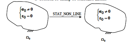
Figure 3.1: Checking the validity of the initial constraint field.

Given the difficulty of validating the implemented formulation, it is currently not legal to combine a pre-deformation (via the keyword PRE_EPSI of the AFFE_CHAR_MECA operator) and an initial stress.

3.5.3. Operand DEFORMATION#

This keyword makes it possible to define the hypotheses used to calculate the deformations. For more details on deformation formalisms, see paragraph DEFORMATIONde [U4.51,11].

To begin with, the quantities calculated by CALC_G_XFEMsont are defined only in small deformations. It is therefore not possible to use formalism other than PETIT, GROT_GDEP or PETIT_REAC for CALC_G_XFEMun. If this is the case, the calculation stops in error.

Then, in theory, there must be coherence between the deformation formalisms used for the mechanical calculation itself and the post-processing that we are talking about here. This would therefore mean that the mechanical calculations themselves must be carried out with the formalisms PETIT, GROT_GDEP or PETIT_REAC only. However, we leave the possibility of carrying out post-processing in small deformations (PETIT) based on the result of a mechanical calculation carried out with another formalism (for example GDEF_LOG). In this case, an alarm is issued, and it is up to the user to decide whether the result provided makes sense or not. To perform a more reliable calculation of the energy return rate in large deformations, it is recommended to use the aperture equivalence method presented briefly in U2.05.01.

◊ DEFORMATION =

/”PETIT”: the deformations used in the behavior relationship are the linearized relationships. This means that we remain on the Small Perturbations Hypothesis: small displacements, small rotations and small deformations. In this case, the calculations of the quantities are legal and validated. This option is the only option available for non-meshed cracks.

/”GROT_GDEP”: Allows you to treat large rotations and large displacements, but while remaining in small deformations

/”PETIT_REAC”: available only in incremental behavior, it is an approximation of large deformations for which the deformation increments are calculated in the current geometry (updated). It is only valid for small increments and for low rotations [U4.51.11].

3.5.4. Operands TOUT/GROUP_MA#

/GROUP_MA = lgrma,

Specify the meshes or nodes on which the behavioral relationship is used.

3.5.5. Behavioral relationship available for each option#

		“ CALC_G “	“ CALC_K_G “
COMPORTEMENT	“ ELAS “	“PETIT” “GROT_GDEP”	“PETIT”
	“ ELAS_VMIS_LINE “ “ ELAS_VMIS_TRAC “ “ ELAS_VMIS_PUIS “	“PETIT” “GROT_GDEP”	not available.

Table 3.6.4-a: Availability, by option, of behavioral relationships.

3.6. Operand OPTION#

♦ OPTION =/'CALC_G',

/”CALC_K_G”,

3.6.1. OPTION = “CALC_G” [R7.02.01] and [R7.02.03]#

It allows the calculation of the energy restoration rate \(G\) by the theta method in 2D or in local 3D for a linear or non-linear thermo-elastic problem.

In 2D, for modeling AXIS, you must divide the result obtained by the radius at the bottom of the crack, see § 4.2.

3.6.2. OPTION = “CALC_K_G” [R7.02.05]#

This option calculates in 2D and 3D the recovery rate \(G\) and the stress intensity coefficients \({K}_{1}\), \({K}_{2}\) and \({K}_{3}\) in plane linear thermo-elasticity by the singular field method (use of the bilinear form of \(G\), [R7.02.05]).

Notes:

For this option, only linear elastic calculations with no initial state or linear elastic calculations with initial stress are available.
For this 2D option, if INFO is 2, the calculation and printing (in the file MESSAGE) of the crack propagation angle is generated. This angle, calculated according to 3 criteria ( \(\mathrm{K1}\) or \(G\) maximum, \(\mathrm{K2}\) minimum) according to the formulas of AMESTOY, BUI and DANG - VAN [R7.02.05 §2.5], is given to within 10 degrees.

3.7. Keyword LISSAGE#

The field of application of this keyword is limited to the local 3D case.

3.7.1. Operand LISSAGE_THETA#

◊ LISSAGE_THETA =/'LEGENDRE' [DEFAUT]

/”LAGRANGE”

The trace of the theta field on the crack background can be discretized either according to the base of the first \(N\) Legendre polynomials (“LEGENDRE”), or according to the shape functions associated with the discretization of the crack background (“LAGRANGE”) [R7.02.01].

LISSAGE_THETA =” LEGENDRE “: \(\theta (s)\) is discretized on the basis of Legendre polynomials \({\gamma }_{j}(s)\) of degree \(j\) (\(0<j<{\mathit{Deg}}_{\mathit{max}}\)) where \({\mathit{Deg}}_{\mathit{max}}\) is the maximum degree given under the keyword DEGRE (between 0 and 7).

LISSAGE_THETA =” LAGRANGE “: \(\theta (s)\) is discretized on the shape functions of the node \(k\) of the crack bottom: \({\phi }_{k}(s)\).

3.7.2. Operand LISSAGE_G#

LISSAGE_G =/”LEGENDRE”, [DEFAUT] /”LAGRANGE”, /”LAGRANGE_NO_NO”

\(G(s)\) can be discretized either according to Legendre polynomials (“LEGENDRE”), or according to the shape functions of the nodes at the bottom of the crack (“LAGRANGE”). The “LAGRANGE_NO_NO” method is derived from the LAGRANGE - LAGRANGE method but it is simplified [R7.02.01].

If the smoothing of theta by Legendre polynomials was retained from the previous keyword, then the smoothing of \(G\) must also be of the Legendre type.

The options available in*Aster* are summarized in the following table:

		Theat
		Polynomials of LEGENDRE	Shape features
\(G(s)\)	Polynomials of LEGENDRE	LISSAGE_THETA = “LEGENDRE” LISSAGE_G = “LEGENDRE”
\(G(s)\)	Shape features		LISSAGE_THETA = “LAGRANGE” LISSAGE_G = “LAGRANGE” or “LAGRANGE_NO_NO”

3.7.3. Operand DEGRE#

◊ DEGRE = n

\(n\) is the maximum degree of the Legendre polynomials used for the decomposition of the \(\theta\) field at the bottom of the crack [§3.12] (when LISSAGE_THETA =” LEGENDRE “).

By default \(n\) is assigned to 5. The value of \(n\) must be between 0 and 7.

If we use the discretizations LISSAGE_THETA =” LAGRANGE “and LISSAGE_G =” “and =” LEGENDRE “, we must have \(n<\mathrm{NNO}\), where \(\mathrm{NNO}\) is the number of knots at the bottom of the crack [R7.02.01 §2.3].

Tips on straightening:

it is difficult to give preference to one or the other straightening method. In principle, both give equivalent numerical results. However, smoothing type “LAGRANGE “is slightly more time consuming CPU than smoothing type” LEGENDRE “* ;
Type smoothing” LEGENDRE “is sensitive to the maximum degree of the polynomials chosen. The maximum degree should be defined according to the number of knots at the bottom of the crack* NNO. If \(n\) is too big compared to \(\mathit{NNO}\) the results are poor [U2.05.01 §2.4];
oscillations may occur with smoothing type “ LAGRANGE “, especially if the mesh has quadratic elements or if the crack is not meshed. If the mesh is radiant at the bottom of the crack (mesh crack), it is then recommended to define crowns R_ INFet R_ SUPcoïncidant with the borders of the elements. A smoothing type “ LAGRANGE_NO_NO “makes it possible to limit these oscillations;
for meshed and non-meshed cracks, when using smoothing type “LAGRANGE “it is recommended to use the operand NB_POINT_FOND to ensure an equal distribution of the calculation points at the bottom of the crack. The choice of a ratio of the order of 5 between the total number of points at the bottom of the crack (to be found in the information printed in the message file by the command DEFI_FISS_XFEM ) and the number of calculation points seems appropriate to limit oscillations;
the use of at least two types of smoothing with several integration crowns and the comparison of the results is **essential in order to verify the validity of the model.*

3.8. Operand CHAM_THETA#

◊ CHAM_THETA = /CO ('cham_theta') [evol_noli]

An evol_noli concept that contains the theta field calculated in the operator (see the reference documentation to know how this field is calculated). This concept contains one cham_no (fields at the nodes) in 2D and several in 3D (depending on the options used for smoothing). In the 3D case, there is one fiel_no per moment in the evol_noli result data structure. This time has no physical meaning, it only allows you to "tidy up" the various fields in the evol_noli data structure.

3.9. Operand TITRE#

◊ TITRE = title

[U4.03.01].

3.10. Operand INFO#

◊ INFO =/1, [DEFAUT]

/2,

Message level in file “MESSAGE”.

3.11. Table produced#

The CALC_G_XFEM command generates a table-like concept.

This table is defined as follows for options CALC_G and CALC_K_G:

In any case	Depends on the calculation performed		In 2D and local 3D only			In local 3D
NUME_FOND	NUME_CAS	NOM_CAS		COOR_X	COOR_Y	COOR_Z	NUM_PT	ABSC_CURV
	NUME_MODE
	NUME_ORDR	INST

Table 3.11-1: Table obtained with CALC_G (1)

In any case	CALC_K_G			CALC_K_G in local 3D
G	K1	K2	G_ IRWIN	K3

Table 3.11-2: Table obtained with CALC_G (2)

\({G}_{\mathrm{IRWIN}}\), is the energy recovery rate obtained from the stress intensity factors \({K}_{1}\) and \({K}_{2}\) (and \({K}_{3}\)) with the following formulas:

\({G}_{\mathrm{IRWIN}}=\frac{1}{E}({K}_{I}^{2}+{K}_{\mathrm{II}}^{2})\) in plane constraints

\({G}_{\mathrm{IRWIN}}=\frac{(1-{\nu }^{2})}{E}({K}_{I}^{2}+{K}_{\mathrm{II}}^{2})\) in plane and axi-symmetric deformations

\({G}_{\mathrm{IRWIN}}=\frac{(1-{\nu }^{2})}{E}({K}_{I}^{2}+{K}_{\mathrm{II}}^{2})+\frac{{K}_{\mathrm{III}}^{2}}{2\mu }\) in 3D

with \(E\) Young’s modulus and \(\nu\) Poisson’s ratio and \(\mu =\frac{E}{2(1+\nu )}\). The comparison between \(G\) and \({G}_{\mathrm{IRWIN}}\) makes it possible to ensure the consistency of the results: too large a difference should lead to the verification of the calculation parameters (mesh refinement, choice of crowns for theta, smoothing in 3D…).

The IMPR_TABLE [U4.91.03] command allows you to print the results in the desired format.