3. Operands#
3.1. Operand MAILLAGE#
♦ MAILLAGE = my
ma: name of the mesh on which we will define the crack. This mesh is necessarily a 2D or 3D mesh.
Attention, quadratic X- FEM elements lack robustness (especially in 3D) we recommend using linear X- FEM elements. So it is preferable that MA be a linear mesh.
3.2. Definition of a grid to be associated with the crack#
An auxiliary grid may be associated with the crack:
or by giving a grid mesh (see § 3.2.1),
or by giving a crack already associated with a previous grid (see § 3.2.2),
In the case of using the upwind method in PROPA_FISS (doc U4.82.11), its use is almost mandatory.
This keyword is typically used following a refinement by Homard of the mesh where the crack was defined.
3.2.1. Operand MAILLAGE_GRILLE#
◊ MAILLAGE_GRILLE = magri [mesh]
magri: name of the grid mesh to be associated with the crack
This operand is used to associate the magri grid mesh with the crack. The two level functions (level set) and their gradients are calculated both on the mesh ma given by MAILLAGE (see § 3.1) and on the magri mesh according to the method chosen by DEFI_FISS (see § 3.4) and they are stored with the crack. Therefore several cracks can be defined on the same magri grid.
The magri mesh is created by the operator DEFI_GRILLE [U4.24.02].
The auxiliary grid used must extend only over the predicted crack propagation zone so as to be able to correctly represent the bottom of the crack during the entire propagation simulation. It may be partly outside the ma grid (keyword MAILLAGE, see § 3.1) and no relationship exists between this mesh and that of the magri grid. In the presence of several cracks and with a different grid use for each, the grids are independent and can be partially or totally superimposed. In this case it is also possible to use a single grid for all the cracks.
3.2.2. Operand FISS_GRILLE#
In the case where we have defined a crack on a mesh with an associated grid and where we want to redefine it on another mesh without changing the grid, we can save calculation time by avoiding recalculating the level functions on the grid. In fact, in this case the level functions defined on the grid do not change.
This is always the case when using Lobster on the mesh where the crack was defined because the grid is not affected by the Lobster changes and the level functions defined initially do not change. We can therefore redefine the same crack on the refined mesh with the same associated grid by calculating the level functions only on the mesh and keeping them the same on the grid.
We specify the fiss_orig crack that was defined before. The grid already present is associated with the new crack and the fields at the calculated nodes that define the level functions and their gradients are copied onto the grid for the new crack. This is equivalent to defining the fiss_orig crack on the new mesh using the same grid all the time.
Note:
No check can be made on the consistency between the crack that will be defined by DEFI_FISS (see § 3.4 ) and the one that was defined on the grid fiss_orig.
3.3. Operand TYPE_DISCONTINUITE#
/”COHESIF” /”INTERFACE”
By default, a crack is defined. However, it is possible to define an interface (to treat the case of 2 solids in contact, or underthicknesses,…).
In the case where TYPE_DISCONTINUITE = “FISSURE”, the data structure produced is enriched with two tables named “FOND_FISS” and “NB_FOND_FISS” that can be retrieved using the RECU_TABLE command. The “NB_FOND_FISS” table contains a single value corresponding to the number of crack bottoms. The table therefore contains a single column (named NOMBRE) and a single row. Table “FOND_FISS” contains the list of the coordinates of the points of all the crack bottoms. This table has 6 columns:
the first column (“NUME_FOND”) corresponds to the number of the crack bottom,
the next column (“NUM_PT”) corresponds to the number of the crack bottom point, this number is local to the current crack bottom,
the next column (“ABSC_CURV”) corresponds to the value of the curvilinear abscissa along the current crack bottom,
the next 3 columns (“COOR_X”, “COOR_Y” and “COOR_Z”) correspond to the coordinates of the point.
The type of discontinuity COHESIFpermet to have information on the propagation front (due to the data mentioned above and the second level function) in order to transmit it to propagation or tracking algorithms for the cracked surface. On the other hand, unlike type FISSURE, it does not contain information related to advanced enrichment, since the latter does not need to be in the presence of cohesive forces. Indeed, it is important to note that for discontinuity type COHESIF, the propagation front does not coincide with the end of Heaviside enrichment, which can cross the entire structure. The initial front must therefore be given independently, using the keyword GROUP_MA_BORD.
3.4. Keyword DEFI_FISS#
♦ DEFI_FISS = _F
The keyword factor DEFI_FISS allows you to define a crack or an interface in 4 different ways:
or from two groups of meshes (see § 3.4.1);
or from two analytical functions (see § 3.4.2);
or from a catalog of predefined shapes (see § 3.4.3);
or from existing fields (see § 3.4.4).
3.4.1. Definition of the crack by groups of cells#
If we have a crack (or an interface) that is already meshed, then we can define the crack by giving two groups of elements: GROUP_MA_FISS and GROUP_MA_FOND. This mesh may be independent of the mesh of the structure.
/♦ GROUP_MA_FISS = Grma
.
with GRMA single group of elements.
This group of elements corresponds to only one of the lips of the crack (lower or upper lip). This group of elements should be oriented. In the case of lips that are not perfectly glued, the fact of choosing one side will have a slight influence on the local base of the crack base, an influence that is even greater as the angle between the two lips is important. For the 2D case, the program sorts the GROUP_MA_FISS cells so as to have a group of elements that are contiguous regardless of the starting group. It is therefore not necessary to give a group of elements that follow one another.
66/ GROUP_MA_FOND = Grma
with GRMA single group of elements.
This operand is used to define the crack background. For interfaces, GROUP_MA_FOND is not a step.
In 2D, GROUP_MA_FOND is a group of elements point.
3.4.2. Definition of the crack by analytical functions#
The main advantage of this operator is the possibility of defining a crack without it necessarily being meshed. In this case, the crack is defined using two level functions (level sets). The first level set (called « normal » level set) is the one that allows the surface of the crack to be characterized. We therefore fill in FONC_LN with a real function of \(X\), \(Y\) and \(Z\) defined beforehand by the FORMULE operator. The surface of the crack will then be the iso-zero for this function. The second level set (called the « tangent » level set) is the one that makes it possible to characterize the crack background. We therefore fill in FONC_LT with a real function of \(X\), \(Y\) and \(Z\) defined beforehand by the FORMULE operator. The iso-zero trace of FONC_LT in the crack plane is the crack background. The crack points are then characterized by FONC_LN = 0 and FONC_LT < 0, while the crack background is characterized by FONC_LN = 0 and FONC_LT = 0.
For interfaces, FONC_LT is not a step.
/♦ FONC_LN = so,
.
with therefore a function or formula defined previously.
* FONC_LT = so,
.
with therefore a function or formula defined previously.
Note:
For a crack, it is essential that the level sets are the true distance functions, so you cannot define an elliptical crack by:
LN= FORMULE (NOM_PARA =( “X”, “Y”, “Z”), VALE =”Z-H”)
LT= FORMULE (NOM_PARA =( “X”, “Y”, “Z”), VALE =” (X/a) ²+ (Y/b) ²-1”)
where a and b would be the semi-major and semi-minor axes of the ellipse. In fact, the LT*function is not the distance to the ellipse. The function distance to an ellipse is not expressed using usual functions. To introduce such a crack, it is necessary to use the 3*th method: pre-defined shapes.
For interfaces, any level set function is possible, and it is not necessary to introduce the real distance function.
Note:
To date nothing would prohibit having a level set that defines several closed crack bottoms (for example several « penny-shaped » cracks). Under these conditions, a call to DEFI_FISS_XFEM could then define several cracks. This possibility is forbidden: each command DEFI_FISS_XFEM *defines only one crack. It is therefore not**possible to define several closed funds OR a closed fund plus one or more open funds. *
Note:
Pay attention to the sign FONC_LT, always remember that the crack is defined on the side FONC_LT < 0.
3.4.3. Definition of the crack by a catalog of predefined shapes#
There is a catalog of pre-defined crack/interface shapes. The choice of shape depends on the dimension of the mesh (2D or 3D). Possible choices are listed in the.
Cracks |
Interfaces |
|
2D |
SEGMENT, DEMI_DROITE |
RECTANGLE, ENTAILLE |
3D |
ELLIPSE, RECTANGLE, CYLINDRE, DEMI_PLAN |
Table 3.4.3-1 : Catalog of predefined shapes
For each shape, specific geometric characteristics must be given.
/♦ FORM_FISS = form,
3.4.3.1. FORM_FISS = “ELLIPSE”#
Case of an elliptical plane crack in 3D or an elliptical inclusion in 2D. You must enter the length of the semi-major axis with the keyword DEMI_GRAND_AXEet and the length of the semi-minor axis with the keyword DEMI_PETIT_AXE. To characterize the plane of the ellipse, we must fill in the center of the ellipse with the keyword CENTRE and the coordinate system of the plane with the keywords VECT_X and VECT_Y. The vector VECT_X corresponds to the axis of the ellipse along which we define the length \(a\) given under the keyword DEMI_GRAND_AXE, and the vector VECT_Y corresponds to the axis of the ellipse along which we define the length \(b\) given under the keyword DEMI_PETIT_AXE.
Note:
Whether you choose \(0<b⩽a\) or \(0<a⩽b\), VECT_Xreste always associated with DEMI_GRAND_AXEet VECT_Yreste always associated with DEMI_PETIT_AXE.
In the case of a crack, you can also specify which side the crack is on (inside or outside the ellipse) using the keyword COTE_FISS. The represents an elliptical crack/inclusion, with a semi-major axis \(a\), a semi-minor axis \(b\), and a center \(C\). The vector \(\vec{{e}_{1}}\) corresponds to the keyword VECT_Xet the vector \(\vec{{e}_{2}}\) corresponds to the keyword VECT_Y.
♦ DEMI_GRAND_AXE = a,

♦ DEMI_PETIT_AXE = b,

♦ CENTRE = (Cx, Cy, Cz),

♦ VECT_X = (e1x, e1y, e1z),

♦ VECT_Y = (e2x, e2y, e2z),

◊ COTE_FISS =/'IN',

/'OUT',


.. image:: images/100000000000021A00000199753A61C8D96C7378.png
    :width: 2.8035 in
    :height: 2.1299 in


.. _RefImage_100000000000021A00000199753A61C8D96C7378.png:


Figure 3.4.3.1-1: Diagram of an elliptical crack/inclusion
3.4.3.2. FORM_FISS = “RECTANGLE”#
Case of a flat rectangular crack in 3D, or of a rectangular inclusion in 2D, with the possibility of rounded corners. It is a form similar to the ellipse, you must enter the same keywords: the value of the semi-major axis (or half-length) with the keyword DEMI_GRAND_AXEet the value of the semi-minor axis (or half-width) with the keyword DEMI_PETIT_AXE. To characterize the plane of the rectangle, we must fill in the center of the rectangle with the keyword CENTREet the coordinate system of the plane. The semi-major axis corresponds to vector VECT_Xet the semi-minor axis corresponds to vector VECT_Y. In addition, in the case of a crack, you can specify on which side the crack is located (inside or outside the rectangle) by the keyword COTE_FISS. The only additional keyword compared to the ellipse shape is the one used to give the value of the radius of the fillet for rounded corners (RAYON_CONGE). The represents a rectangular-shaped crack/inclusion with rounded corners, with a semi-major axis \(a\), a semi-minor axis \(b\) and a center \(C\). The vector \(\overrightarrow{{e}_{1}}\) corresponds to the keyword VECT_Xet the vector \(\overrightarrow{{e}_{2}}\) corresponds to the keyword VECT_Y. The radius for rounded corners is \(r\). By default the leave radius is zero.
♦ DEMI_GRAND_AXE = a,

♦ DEMI_PETIT_AXE = b,

◊ RAYON_CONGE = r,

♦ CENTRE = (Cx, Cy, Cz),

♦ VECT_X = (e1x, e1y, e1z),

♦ VECT_Y = (e2x, e2y, e2z),

◊ COTE_FISS =/'IN',

/'OUT',


.. image:: images/10000000000002b4000001 ED3FABE66D4C27D9EC .png
    :width: 3.3047 in
    :height: 2.3543 in


.. _refImage_10000000000002b4000001 ED3FABE66D4C27D9EC .png:


Figure 3.4.3.2-1: Diagram of a rectangular crack/inclusion with rounded corners
3.4.3.3. FORM_FISS = “CYLINDRE”#
Case of a three-dimensional cylindrical crack with elliptical cross section. To characterize the bottom (elliptical) of the crack, you must enter the length of the semi-major axis with the keyword DEMI_GRAND_AXEet the length of the semi-minor axis with the keyword DEMI_PETIT_AXE. We must also fill in the center of the ellipse with the keyword CENTREainsi as the coordinate system of the plane (VECT_X, VECT_Y). Note: the semi-major axis corresponds to the vector VECT_Xet the semi-minor axis corresponds to the vector VECT_Y. The generator of the cylinder and the direction of potential propagation of the crack are given by the vector product of VECT_XparVECT_Y. This cylinder is semi-infinite along this axis. The illustrates a cylinder-type crack with a semi-major axis :math:`a`, a semi-minor axis :math:`b` and a center :math:`C`. The vector :math:`\overrightarrow{{e}_{1}}` corresponds to the keyword VECT_X and the vector :math:`\overrightarrow{{e}_{2}}` corresponds to the keyword VECT_Y.


♦ DEMI_GRAND_AXE = a,

♦ DEMI_PETIT_AXE = b,

♦ CENTRE = (x0, y0, z0),

♦ VECT_X = (vxx, vxy, vxz),

♦ VECT_Y = (vyx, vyy, vyz),


.. image:: images/100000000000017A000002165760B1809E190F4F.png
    :width: 1.9689 in
    :height: 2.7799 in


.. _RefImage_100000000000017A000002165760B1809E190F4F.png:


Figure 3.4.3.3-1: Diagram of a cylinder crack
3.4.3.4. FORM_FISS = “ENTAILLE”#
Case of a notch-type inclusion in 2D. This is a particular case of the inclusion of the rectangle type with rounded corners in the where the half-height is equal to the radius of leave. To define the notch you must enter the value of the half-length with the keyword DEMI_LONGUEUR, the value of the radius of the fillet with the keyword RAYON_CONGE and the center of the notch with the keyword CENTRE. In addition, the direction of the cut is given by the keywords VECT_Xet VECT_Y. The represents a notch inclusion, with a half-length :math:`a`, a fillet radius :math:`r`, and a center :math:`C`. The vector :math:`\overrightarrow{{e}_{1}}` corresponds to the keyword VECT_Xet the vector :math:`\overrightarrow{{e}_{2}}` corresponds to the keyword VECT_Y.


♦ DEMI_LONGUEUR = a,

♦ RAYON_CONGE = r,

♦ CENTRE = (Cx, Cy, Cz),

♦ VECT_X = (e1x, e1y, e1z),

♦ VECT_Y = (e2x, e2y, e2z),


.. image: images/1000000000000242000001 BCBA7E9AD54A61E488 .png
    :width: 3.3047 in
    :height: 2.5382 in


.. _refImage_1000000000000242000001 BCBA7E9AD54A61E488 .png:


Figure 3.4.3.4-1: Diagram of a rectangular crack/inclusion with rounded corners
3.4.3.5. FORM_FISS = “DEMI_PLAN”#
Case of a crack defined by a half-plane. PFON refers to a point at the bottom of a crack. NORMALE defines the normal to the crack's half-plane and DTAN provides a vector in the crack plane, orthogonal to the bottom, and directed in the direction of potential propagation. The represents a half-plane crack defined by :math:`P` a point at the bottom, the vector :math:`\overrightarrow{{e}_{1}}` corresponds to the keyword DTAN and the vector :math:`\overrightarrow{{e}_{2}}` corresponds to the keyword NORMALE.


♦ PFON = (Px, Py, Pz),

♦ DTAN = (e1x, e1y, e1z),

♦ NORMALE = (e2x, e2y, e2z),
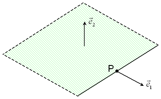
Figure 3.4.3.5-1 : diagram of a half-plane crack
3.4.3.6. FORM_FISS = “SEGMENT”#
Case of a 2D crack defined by a segment. PFON_ORIG and PFON_EXTR refer to the ends of the segment. This is a 2D segment-type crack where :math:`\mathit{P1}` designates the point of origin PFON_ORIG and :math:`\mathit{P2}` the end point PFON_EXTR.


♦ PFON_ORIG = (P1x, P1y, P1z),

♦ PFON_EXTR = (P2x, P2y, P2z),
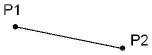
Figure 3.4.3.6-1 : diagram of a segment-type 2d crack
3.4.3.7. FORM_FISS = “DEMI_DROITE”#
Case of a 2D crack defined by a half-line. PFON refers to the point at the bottom of the crack. DTAN corresponds to a direction vector of the half-line oriented in the direction of potential propagation. This is a 2D half-line crack for which \(P\) is the bottom point (PFON) and has a direction vector \(\overrightarrow{{e}_{1}}\) (DTAN).
♦ PFON = (x0, y0, z0),

♦ DTAN = (e1x, e1y, e1z),
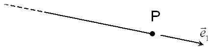
Figure 3.4.3.7-1 : diagram of a 2D half-right crack
If form = DROITE
Case of a straight interface in a defined 2D structure. POINT refers to a point on the interface. DTAN corresponds to a direction vector of the line. Orientation is not important.
♦ POINT = (x0, y0, z0),

♦ DTAN = (vtx, vty, vtz),
3.4.4. Definition of the crack by rereading fields at existing nodes#
/♦ CHAM_NO_LSN = ch_lsn, [cham_no]
◊ CHAM_NO_LST = ch_lst, [cham_no]
The ch_lsn and ch_lst fields are fields with existing nodes. They must have been created on the same mesh that the mesh given me as input under the keyword MAILLAGE (see § 3.1).
These nodal fields can be obtained successively by reading a table (LIRE_TABLE), then by creating the field by extracting the table (CREA_CHAMP/OPERATION =” EXTR “).
They could also be generated in a mesh refinement stage (MACR_ADAP_MAIL/MAJ_CHAM).
3.4.5. Definition of the initial propagation front for a cohesive crack#
/♦ GROUP_MA_BORD = group_ma, [l_gr_mesh]
For a propagation study in the presence of cohesive forces, it is necessary to give the initial propagation front, that is to say the line from which the cracking starts. It is generally a corner of the structure, or a bottom notch, or more generally a line located on an edge. It is given either in the form of a 1D mesh group if it is meshed, or in the form of a group of 2D edge cells, whose intersection with the normal level-set will provide the initial propagation front.
3.4.6. Examples#
if you want to define a bar that is cracked right through and through in its plane at height \(z=H\) (see [Figure 3.2-a], on which the crack is hatched):
LN= FORMULE (NOM_PARA =( “X”, “Y”, “Z”), VALE =”Z-H”);
LT= FORMULE (NOM_PARA =( “X”, “Y”, “Z”), VALE =”Y-a”);
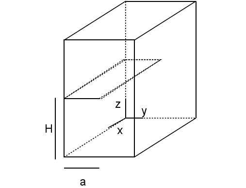
Figure 3.2-a: Cracked bar
if we want to define an elliptical crack in an infinite massif in a plane at the height \(z=H\) (see [Figure 3.2-b], on which the crack is hatched):
DEFI_FISS = _F (FORM_FISS = 'ELLIPSE',
DEMI_GRAND_AXE = a, DEMI_PETIT_AXE = b, CENTRE = (0, 0, H), VECT_X = (1, 0, 0), VECT_Y = (0, 1, 0), COTE_FISS = “IN”,),
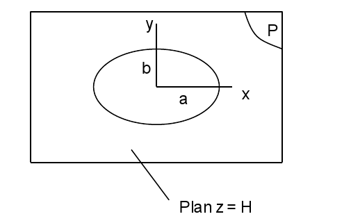
Figure 3.2-b: Elliptical crack
3.5. Operand GROUP_MA_ENRI#
This operand makes it possible to know the zone on which the enrichment procedure will be carried out. The enriched nodes must belong to this mesh group.
If GROUP_MA_ENRI is not entered, then the enrichment procedure will be carried out on the entire mesh given to me as input under the MAILLAGE keyword (see § 3.1)
A use of this keyword therefore makes it possible to delimit the zone of enrichment, and therefore of the crack. The following example shows an elliptical crack in a hollow cylinder. The crack is defined by the data of groups of cells (keywords GROUP_MA_FISS and GROUP_MA_FOND). Two level sets are deduced from this, considering an extension of the crack base by continuity. If the enrichment zone contains the entire structure, then this leads to a crack in the right part of the cylinder, which is not what we want at all. To solve this problem, all you have to do is limit the enrichment zone and fill in the keyword GROUP_MA_ENRI with the cells in the left half of the cylinder for example.
3.6. Operand CHAM_DISCONTINUITE#
This keyword allows you to choose the type of fields to be enriched. At the moment, only the movement field can be enriched.
3.7. Operands TYPE_ENRI_FOND, RAYON_ENRI, NB_COUCHES#
◊ TYPE_ENRI_FOND =/'GEOMETRIQUE' [DEFAUT]
/”TOPOLOGIQUE”
This keyword allows you to choose the type of enrichment at the bottom of the crack. Topological enrichment (a single layer) is activated if TYPE_ENRI_FOND = “TOPOLOGIQUE”. Geometric enrichment (multiple layers) is activated if TYPE_ENRI_FOND = “GEOMETRIQUE” (for more information about the effects of enrichment on the quality of results, see [R7.02.12] and [U2.05.02]). Geometric enrichment is driven by the keywords RAYON_ENRI and NB_COUCHES.
◊ RAYON_ENRI = Renri, [R]
This keyword can only be entered if TYPE_ENRI_FOND = “GEOMETRIQUE”. If this operand is entered, it makes it possible to specify a Renri geometric criterion such that all the nodes whose distance from the crack bottom is less than this criterion will be enriched by the singular functions. This enrichment is called « geometric ». Studies have shown that such enrichment greatly improves the accuracy of calculations, especially when the mesh is refined at the bottom of the crack. It is advisable to choose Renri approximately equal to 1/10 of the crack length. Conditioning is very little affected by the use of geometric enrichment thanks to the introduction of vector enrichment functions at the bottom of the crack [R7.02.12].
To avoid the inconveniences caused by an excessive radius of enrichment (increase in the cost of calculation), we can define the area to be enriched by stipulating the number of layers of elements to be enriched around the bottom of the crack in place of the radius of enrichment in place of the radius of enrichment.
# If RAYON_ENRI = None
◊ NB_COUCHES =/2, [DEFAUT]
/N, [I]
If RAYON_ENRI is not entered (and TYPE_ENRI_FOND = “GEOMETRIQUE”), then NB_COUCHES is the number of element layers to be enriched (2 by default). The use of a large number of layers only impacts the calculation cost, especially in 3D.
3.8. Operand JONCTION#
# If MAILLAGE_GRILLE = None,

◊ JONCTION = _F (
♦ FISSURE = (fiss1, fiss2,…, fissi), [l_fiss_xfem]
♦ POINT = (Px, Py, Pz), [L_r]
This operand makes it possible to define one or more junctions between a crack and other cracks that already exist. These other cracks are then considered as root cracks: you must have already defined them beforehand by calls to DEFI_FISS_XFEM.
A list of root cracks is entered in the keyword FISSURE. All of these root cracks will be taken into account when defining the current crack. The key word POINTdoit be given in the field where you want the crack to be defined. An example is provided in Figure 3.7-a. In this figure, it is considered that crack 3 was initially defined to cut the domain vertically. We introduce the keyword JONCTIONafin to connect it to cracks 1 and 2. The three configurations of the figure can be obtained according to the choice of position given in the keyword POINT.
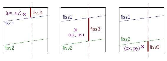
Figure 3.8-1: Example of the definition of the fiss3 crack, for the mother cracks \(\mathit{fiss1}\) and \(\mathit{fiss2}\), according to the point \((\mathit{px},\mathit{py})\) chosen.
You have to be careful when using the JONCTION operand: the crack will then no longer only be represented by its normal and tangent level sets, but it will also depend on the root cracks. This can be a problem if you want to use operators like RAFF_XFEM, which only allow for the definition of a crack by level-sets. Likewise, the graphical representation of the iso-zero of the level sets is not sufficient, it is preferable to go through the post-processing operations via the operator POST_MAIL_XFEM.
An example of configuration is shown. In this example, cracks are identified that another crack connects to. So for crack \(N=3\), we have \(K=2\) where K is the set of cracks to which 3 connects. Similarly for crack \(N=5\), \(K=[\mathrm{3,4}]\) is deduced. Fissure 5 is therefore defined from the junction operand and from the two cracks 3 and 4. Fissure 3 is itself defined previously from the junction operand acting on crack 2, which is itself defined from the junction operand acting on crack 1. The hierarchy tree is therefore used to establish the order of definition of the various cracks (2 from 1, 3 from 2, 4 from 1 and 5 from 3 and 4).
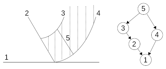
Figure 3.8-2 : Fissure network on the left, hierarchy tree on the right showing who is plugging in and allowing to establish order relationships for crack definitions and the use of the operand JONCTION .
The junction operator makes it possible to establish an order relationship for a mesh that sees \(N\) cracks. We will thus distinguish on the two right-hand hierarchy trees. In the rightmost tree, cracks 1 and 2 are close enough for a cell that sees crack 3 to also see cracks 1 and 2: we therefore decide to connect crack 3 to cracks 2 and 1, but to also use the junction operand to indicate that crack 2 is connected to crack 1. For the other tree, a mesh sees at most 2 cracks (no mesh then sees both cracks 1, 2 and 3) and in this case crack 3 simply connects to cracks 2 and 1 which are no longer connected to each other.
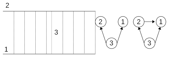
Figure 3.8-3 : Network of cracks on the left, hierarchy trees on the right.
The rightmost hierarchy tree indicates that crack 2 cannot be defined independently of crack 1 because it is too close to this last one (a mesh that sees crack 3 then also sees cracks 1 and 2).
3.9. Operand INFO#
/ 1 :
|
Print on the file “MESSAGE”
|
/ 2 :
|
same impressions as 1 + prints
|
/ 3 :
|
same impression as 2 + impressions
|