3. Operands#

3.1. Operand RESULTAT#

♦ RESULTAT = resu

Name of a result concept such as evol_elas, evol_noli, dyna_trans or mode_meca. This operand makes it possible to recover the displacement field (and speed and acceleration for a dynamic calculation).

The model and the material field, which are required for the calculation, are also extracted from the result data structure. The possible calculation options for each type of modeling are listed in the table below.

	Calculation of \(G\)	Calculation of \(K\)	Calculation of \(\mathit{KJ}\)
D_ PLAN/C_ PLAN, D_ PLAN_INCO_UPG	CALC_G (OPTION “G”)	CALC_G (OPTION “K”)	CALC_G (OPTION “KJ”)
AXIS, AXIS_INCO_UPG	CALC_G (OPTION “G”)	CALC_G (OPTION “K”)	CALC_G (OPTION “KJ”)
3D, 3D_ INCO_UPG	CALC_G (OPTION “G”)	CALC_G (OPTION “K”)	CALC_G (OPTION “KJ”)

Table 3.1: Availability, by modeling, of calculation options.

Notes on material properties:

The characteristics of the material, retrieved from the resu data structure, are as follows:

Young’s modulus E,
NU Poisson’s ratio,
thermal expansion coefficient ALPHA (for a thermo-mechanical problem),
elastic limit SY (for a non-linear elastic problem),
slope of the tensile curve D_ SIGM_EPSI (for a nonlinear elastic problem with linear isotropic work hardening).

For the calculation of the energy return rate, these characteristics may depend on the geometry (options “G” and “KJ”) and on the temperature (options” G “and” KJ “). They must be independent of temperature for the calculation of stress intensity factors (option “K”).

The SY and D_ SIGM_EPSI characteristics are only treated for a nonlinear elastic problem with Von Mises work hardening. The calculation of stress intensity coefficients is treated only in linear elasticity.

Note:

For the calculation of stress intensity factors (option “K”), the characteristics must be defined on all materials, including on the edge elements, due to the calculation method [R7.02.05]. To ensure this, it is advisable to do a AFFE = _F (TOUT = “OUI”) in the command AFFE_MATERIAU [U4.43.03], even if it means using the overload rule afterwards.

For incompressible elements (_ INCO_UPG), it is recommended to use STAT_NON_LINEpour to get the results.

The stress intensity factors obtained with option “K” are calculated by evaluating the bilinear form of G with a purely mechanical singular solution (asymptotic Westergaard solution). If a thermo-mechanical problem is solved, the singularity due to the thermal field is then not taken into account.

An indicator of the error due to this approximation can be obtained by evaluating the difference between Get G_ IRWIN. In practice, the quantity \(\frac{∣G-{G}_{\mathit{irwin}}∣}{∣G∣}\) is evaluated at any point at the bottom of the crack, and the arithmetic mean is then calculated. If this average exceeds 50%, it is then estimated that we are outside the scope of validity of the approach. This check is the responsibility of the user.

Bi-material problem:

1st case: We have a bi-material but the crack point is in a single material, cf. Figure 3.1-a. If it is ensured that the crown, defined between the lower radii R_ INF and the upper radius R_ and the upper radius R_ SUP, has elements of the same material as support, the calculation is possible regardless of the option chosen. Otherwise only option “G” is possible.

Figure 3.1-a: Bi-material: 1st case

2ndcas: We have a bi-material where the crack tip is at the interface, cf. Figure 3.1-b. To date, only the option for calculating the energy return rate (option “G”) is available. The calculation of stress intensity coefficients is not possible in this case.

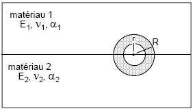
Figure 3.1-b: Bi-material: 2nd case

3.2. Operands TOUT_ORDRE/NUME_ORDRE/LIST_ORDRE/INST//LIST_INST///TOUT_MODE/NUME_MODE//LIST_MODE/FREQ/purpose LIST_FREQ PRECISION CRITERE#

These operands are used with operand RESULTAT.

The operands TOUT_ORDRE, NUME_ORDRE, LIST_ORDRE, INST, LIST_INST are associated with evol_elas, evol_noli or dyna_trans results. See [U4.71.00].

The operands TOUT_MODE, NUME_MODE, LIST_MODE, FREQ, LIST_FREQ are associated with mode_meca results.

3.3. Operand OPTION#

♦ OPTION = | 'G',

“K”,
“G_EPSI”,
“KJ”,
“KJ_EPSI”,

3.3.1. OPTION = “G” [R7.02.01] and [R7.02.03]#

It allows the calculation of the energy restoration rate \(G\) by the theta method in 2D or in local 3D for a linear or non-linear thermo-elastic problem.

For this calculation, the constraint and displacement fields of the result as input to the operator are directly used.

3.3.2. OPTION = “K” [R7.02.05]#

This option calculates in 2D and 3D the stress intensity coefficients \({K}_{1}\), \({K}_{2}\) and \({K}_{3}\) in plane linear thermo-elasticity using the singular field method (use of the bilinear form of \(G\), [R7.02.05]), as well as the quantity \({G}_{\mathrm{IRWIN}}\) (see section 3.9).

Notes:

For this option, only linear elastic calculations with no initial state or linear elastic calculations with initial stress are available.
The calculation of this option is only possible if the lips are initially glued ( CONFIG_INIT =” COLLEE “in DEFI_FOND_FISS [U4.82.01] ) .

3.3.3. OPTION = “G_ EPSI “#

It allows the calculation of the energy restoration rate \(G\) by the theta method in 2D or in local 3D for a linear or non-linear thermo-elastic problem when the constraints are recalculated from the field of displacement and the law of behavior.

This operand is only available in elasticity (linear or not) and without an initial state resulting from the keyword ETAT_INIT (see section 3.7).

Note:

If the laws of behavior used for mechanical calculation and for post-processing are the same - which is normal practice - then the results with or without recalculation of the constraints are identical.

A common practice for taking plasticity into account, however, consists in doing an elastoplastic mechanical calculation, followed by a non-linear elastic post-treatment to calculate of \(G\). If we remain within the validity range of the calculation of \(G\) (radial and monotonic loading), then the results with or without recalculation of the constraints, \(G\) and \(G\text{\_}\mathit{EPSI}\) are identical. As soon as we leave this field of validity, the gap increases.

This option, to be reserved for experienced users, therefore makes it possible to check afterwards that we remain true to the calculation assumptions of \(G\).

3.3.4. OPTION = “KJ”#

It allows the calculation of the stress intensity factor \({K}_{1}\) from the energy recovery rate \(G\) and the Irwin formula (see section 3.9). Therefore, this option only makes sense when loading in mode I.

The method used to calculate the energy return rate \(G\) is identical to that used in the case OPTION = “G”.

Note:

If G is negative at a point, then by convention the command will return KJ = 0 for that point.

3.3.5. OPTION = “KJ_EPSI”#

The method used to calculate the energy return rate \(G\) is identical to that used in the case OPTION = “G_ EPSI “.

Note:

If G is negative at one point, then by convention the command will return KJ_ EPSI = 0 for that point.

3.4. Keyword TITRE#

For operand TITRE, you can refer to the associated documentation:

◊ TITRE = title

[U4.03.01].

3.5. Keyword THETA#

The theta field is calculated in CALC_G using the FISSURE keyword.

Tips on choosing crowns (in CALC_G):

Avoid using a theta field defined with a lower radius R_ INF nil. The displacement fields are singular at the bottom of a crack and introduce inaccurate results in post-treatment of fracture mechanics.
It is recommended to use the command CALC_G successively with at least three theta fields from different crowns to ensure the stability of the results. In case of significant variation (greater than 5-10%), it is necessary to question whether all the modeling is properly taken into account.
For the option Ken 2D-axisymmetric, the radius of the crowns must be small compared to the radius of the crack bottom to have the best possible precision. It is forbidden to have crowns with a radius greater than the radius of the crack bottom.

3.5.1. Operands FISSURE#

♦/FISSURE = ff,

This operand allows you to define the theta field (s).

ff is the crack bottom defined by the command DEFI_FOND_FISS [U4.82.01] for an open or closed crack bottom (double backgrounds forbidden in CALC_G).

3.5.2. Operand CHAM_THETA#

◊ CHAM_THETA = /CO ('cham_theta') [CO, cham_no_sdaster]

Type COpermet concept of outputting the computed theta field into the operator (see the reference documentation [:ref:`R7.02.01 <R7.02.01>`] for how this field is calculated), whose name is the given character string. This concept contains a cham_no (fields at the nodes) in 2D and 3D.

Type concept cham_no_sdaster allows you to provide a theta field, instead of calculating one in the operator. In this case, the keywords R_ INF, R_ INF_FO,, NB_COUCHE_INF,,, R_ SUP, R_ SUP_FP, NB_COUCHE_SUPne are no longer supported because the necessary information is already provided in the theta field.

3.5.3. Operands R_ INF, R_ INF_FO,, NB_COUCHE_INF,,, R_ SUP, R_ SUP_FO, NB_COUCHE_SUP#

These operands make it possible to calculate the theta field when this one has not been previously determined. They correspond respectively to the lower (R_ INF and R_ and R_ INF_FO) and upper radii of the crowns (R_ SUP and R_ SUP_FO) (scalar or function, in 3D, of the curvilinear abscissa).

The two radii can be introduced either by constant real values that are arguments of simple keywords R_ INFet R_ SUP; or by functions of the curvilinear abscissa on the oriented crack background, which are arguments of the simple keywords R_ INF_FOet R_ SUP_FO.

A few tips are given below. When the radii are not a function of the curvilinear abscissa, the operands R_ INF and R_ SUP are optional. If they are not specified, they are automatically calculated from the maximum h of the mesh sizes connected to the nodes at the crack bottom. These mesh sizes at each bottom node are calculated in command DEFI_FOND_FISS. It was chosen to pose R_ SUP = 4h and R_ INF = 2h. If you choose the value automatically calculated for R_ SUP and R_ INF, you must however ensure that these values (displayed in the .mess file) are consistent with the dimensions of the structure.

Alternatively, it is possible to define the integration crowns of the theta field in terms of the number of layers (NB_COUCHE_INF and NB_COUCHE_SUP). The concept of layers here is based on mesh connectivity (see the reference documentation [R7.02.01] for more details).

In the case of a defect that is initially open and whose bottom is not flat, it is currently not possible to calculate the energy return rate.

3.5.4. Operand DISCRETISATION#

The field of application of this keyword is limited to the 3D case.

3.5.4.1. Operand DISCRETISATION = LINEAIRE#

The trace of the theta field on the crack background is discretized according to the shape functions associated with the discretization of the crack background (“LAGRANGE”) [R7.02.01].

It is possible to reduce the number of background nodes used for a “LINEAIRE” discretization with the following keyword:

◊ NB_POINT_FOND = nbnofo,

By default, the calculation is done on all the nodes at the crack bottom for a mesh crack. If the mesh is free, the number of nodes at the bottom of the crack can be significant, which leads to very long calculation times.

The NB_POINT_FOND operand makes it possible to fix the number of post-processing points in advance, in order to improve the consistency of the results. The \(\mathit{nbnofo}\) points are evenly distributed along the crack bottom.

In the case where the NB_POINT_FOND operand is not specified for a quadratic mesh, a treatment, by smoothing via a « hat » function, is added to remove the strong oscillations on the post-processing of \(G(s)\) or \(K(s)\).

3.5.4.2. Operand DISCRETISATION = LEGENDRE#

The trace of the theta field on the crack background is discretized according to the basis of the first \(N\) Legendre polynomials (“LEGENDRE”), [R7.02.01].

The user can choose the number of polynomials he wants to do the calculation with the following keyword:

◊ DEGRE = n

\(n\) is the maximum degree of the Legendre polynomials used for the decomposition of the \(\theta\) field at the bottom of the crack.

By default \(n\) is assigned to 5. The value of \(n\) must be between 0 and 7.

3.5.4.3. Advice on discretization#

it is difficult to give preference to one or the other straightening method. In principle, both give equivalent numerical results. However, smoothing type “LINEAIRE “is slightly more time consuming CPU than smoothing type” LEGENDRE “* ;
Type smoothing” LEGENDRE “is sensitive to the maximum degree of the polynomials chosen. The maximum degree should be defined according to the number of knots at the bottom of the crack* NNO. If \(n\) is too big compared to \(\mathit{NNO}\) the results are poor [U2.05.01 §2.4];
oscillations may occur with smoothing type “ LINEAIRE “, especially if the mesh includes quadratic elements. If the mesh is radiant at the bottom of the crack (mesh crack), it is then recommended to define crowns R_ INFet R_ SUPcoïncidant with the borders of the elements.
for mesh cracks, when using a smoothing type “LINEAIRE “it is recommended to use the operand NB_POINT_FOND to ensure an equal distribution of the calculation points at the bottom of the crack. The choice of a ratio of the order of 5 between the total number of points at the bottom of the crack (to be found in the information printed in the message file by the command DEFI_FOND_FISS ) and the number of calculation points seems appropriate to limit oscillations;
the use of at least two types of smoothing with several integration crowns and the comparison of the results is **essential in order to verify the validity of the model.*

3.6. Keyword EXCIT and CHARGE/FONC_MULT operands#

◊ FONC_MULT = fmult)

The keyword EXCIT makes it possible to retrieve a list of loaded loads, from commands AFFE_CHAR_MECA or AFFE_CHAR_MECA_F [U4.44.01], and the possible associated multiplier coefficients fmult.

If the EXCITest keyword is not present in the command, the load taken into account is the one extracted from resu. If the load is provided via EXCIT, then that load will be used in CALC_G. If the load provided in EXCITest is different from that in resu (consistency of the name and number of charges, load-function pairs), an alarm is issued and the calculation continues with the loads indicated by the user.

However, if the result is dyna_trans or mode_meca, it is possible to retrieve a list of loads from the resu. Taking these loads into account in the calculation of G therefore requires the keyword EXCIT.

The loads currently supported by the various models and which may make sense in fracture mechanics are as follows:

Volume force: ROTATION, FORCE_INTERNE, PESANTEUR.
Surface force on the lips of the crack: FORCE_CONTOUR (2D), FORCE_FACE (3D), PRES_REP.
Thermal expansion: the temperature is transmitted via AFFE_MATERIAU/AFFE_VARC
Initial deformation: this deformation is transmitted via the command variable EPSA (anelastic deformation) in AFFE_MATERIAU/AFFE_VARC
Pre-deformation: PRE_EPSI (only in the case of a mesh crack, for option G_ EPSI. Apart from this particular configuration, the unloading application PRE_EPSI leads to false results)
In the event of a thermo-mechanical problem, the temperature is transmitted via the material properties (AFFE_MATERIAU/AFFE_VARC/EVOL). Thermal expansion is therefore automatically taken into account in the calculation with CALC_G. The same is true if an initial deformation is transmitted via the command variable EPSA.

Note:

Loads that are not supported by an option are **ignored. To date, the following loads that may make sense in fracture mechanics are not treated:*

FORCE_NODALE
FORCE_ARETE
DDL_IMPO on the lips of the crack
FACE_IMPO
PRE_EPSI except for the only case treated « mesh crack and option G_ EPSI »

It is important to note that the only loads taken into account in a fracture mechanics calculation with method \(\theta\) are those supported by the elements inside the crown, where the vector field theta is non-zero (between R_ INF and R_ and R_ SUP [R7.02.01 §3.3]). The only types of load likely to influence the calculation of \(G\) are therefore volume loads (gravity, rotation), a non-uniform temperature field or forces applied to the lips of the crack.

Attention:

If several loads of the same nature (for example, volume force) appear in the calculation, they are combined together for post-processing. However, it is currently not possible to make this combination if loads FORMULE are present: the calculation then ends in error. *
An exclusion rule is also applied when there is a simultaneous presence of a pre-deformation field (via “PRE_EPSI “) and an initial stress field.
An exclusion rule is also applied when a deformation field initials (via “EPSA “) and an initial stress field are simultaneously present.
An exclusion rule is also applied when there is a simultaneous presence of a pre-deformation field (via “PRE_EPSI” ) and a deformation field initials * (via “ EPSA “) .
It is not possible at this time to associate a load defined based on a FORMULEet a multiplier coefficient ( FONC_MULT ). In this case, the calculation ends in error.
Kinematic loads ( AFFE_CHAR_CINE and AFFE_CHAR_CINE_F ) cannot be taken into account in the calculation.
For the option K , if a loading is imposed on the lips of the crack ( PRES_REP*or*FORCE_CONTOUR), then it is required* **obligatoryto orient their meshes correctly (using* ORIE_PEAU_2D or or*ORIE_PEAU_3D*) prior to calculating K. *
Note that the calculation of CALC_G is available * only for the results of thermo-mechanical calculations in HPP (keyword DEFORMATION = * “ PETIT “) .

3.7. Operand ETAT_INIT#

◊ ETAT_INIT =_F (SIGM = Siefelga)

In the case of an incremental elastic behavior relationship, it is possible to define a non-zero initial stress state.

The use of this keyword first requires the definition of an initial state in the operator STAT_NON_LINElors for the resolution of the calculation to be post-processed by CALC_G.

STAT_NON_LINE allows this definition in two ways (see u4.51.03):

with an initial results-type state, entered under the keyword EVOL_NOLI of the keyword factor ETAT_INIT
with an initial field-type state, filled in under the keywords SIGM/DEPL//VARI/STRX/COHE of the keyword factor ETAT_INIT

To date, post-processing with CALC_Gdes calculations using the keywords EVOL_NOLI/DEPL//VARI/STRX/COHEn is not possible. Only post-processing with CALC_Gdes calculations using the SIGMest keyword is possible.

The initial constraint field provided can be of type SIEF_ELGA, SIEF_ELNO, or SIEF_NOEU in a FEM model.

In all cases, this initial stress field must be self-balanced, in the absence of cracks, with only the boundary conditions. The user must verify that his initial stress field is valid by applying it in the ETAT_INIT keyword of the STAT_NON_LINE operator, with linear elastic behavior (RELATION = “ELAS”), with the only boundary conditions; the mechanical result must be the same stress field without additional deformations (see).

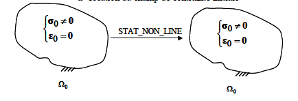
Figure 3.1: Checking the validity of the initial constraint field.

The initial state of the structure can also be represented through a pre-deformation field (via the keyword PRE_EPSI of the AFFE_CHAR_MECA operator). In this case, it is a load included in the result data structure (see section 3.6) and the ETAT_INIT keyword should not be filled in.

Given the difficulty of validating the implemented formulation, it is currently not legal to combine a pre-deformation (via the keyword PRE_EPSI of the AFFE_CHAR_MECA operator) and an initial stress or an initial deformation (via the command variable EPSA of AFFE_MATERIAU/AFFE_VARC) and an initial stress (via the command variable of/) and an initial stress.

3.8. Operand INFO#

◊ INFO =/1, [DEFAUT]

/2,

Message level in file “MESSAGE”.

3.9. Table produced#

The CALC_G command generates a table-like concept.

This table is defined as follows for GetK options:

In any case				In local 2D		In local 3D			In any case
NUME_FOND	INST	NOEUD	NUM_PT	COOR_X	COOR_Y	COOR_Z	ABSC_CURV	ABSC_CURV _ NORM	COMPORTEMENT	TEMPERATURE

Table 3.9-1: Table obtained with CALC_G (1)

CALC_G OPTION G or KJ	CALC_G OPTION K			CALC_K_G in local 3D	CALC_G OPTION KJ
G	K1	K2	G_ IRWIN	K3	KJ

Table 3.9-2: Table obtained with CALC_G (2)

\({G}_{\mathit{IRWIN}}\), is the energy recovery rate obtained from the stress intensity factors \({K}_{1}\) and \({K}_{2}\) (and \({K}_{3}\)) with the following formulas:

\({G}_{\mathrm{IRWIN}}=\frac{1}{E}({K}_{I}^{2}+{K}_{\mathrm{II}}^{2})\) in plane constraints

\({G}_{\mathrm{IRWIN}}=\frac{(1-{\nu }^{2})}{E}({K}_{I}^{2}+{K}_{\mathrm{II}}^{2})\) in plane and axi-symmetric deformations

\({G}_{\mathrm{IRWIN}}=\frac{(1-{\nu }^{2})}{E}({K}_{I}^{2}+{K}_{\mathrm{II}}^{2})+\frac{{K}_{\mathrm{III}}^{2}}{2\mu }\) in 3D

with \(E\) Young’s modulus and \(\nu\) Poisson’s ratio and \(\mu =\frac{E}{2(1+\nu )}\). The comparison between \(G\) and \({G}_{\mathrm{IRWIN}}\) makes it possible to ensure the consistency of the results: too large a difference should lead to the verification of the calculation parameters (mesh refinement, choice of crowns for theta, smoothing in 3D…).

The IMPR_TABLE [U4.91.03] command allows you to print the results in the desired format.