5. Transient response calculation on a modal basis#
Let us consider the finite element model of a linear structure, presenting internal dissipation mechanisms, subject to external forces, which may as well be known a priory (loads) as well as having to be evaluated progressively (shock forces, contact, etc.). In the time domain, the equilibrium relationship is written as:
where \({\mathrm{K}}_{e}\) is the stiffness matrix of the structure, \({\mathrm{D}}_{v}\) the matrix associated with viscous dissipation, and \(\mathrm{M}\) the mass matrix. We also note \(\mathrm{q}\) the vector of degrees of freedom. The term external forces is defined by the product of a force location matrix \(\mathrm{B}\) and a vector \(\mathrm{u}\) specifying the temporal evolution of the excitation. This writing makes it possible to separate the spatial and temporal components of an effort often noted \(\mathrm{f}(t)\). In this case, we will therefore have:
Solving the problem based on the complete model presented in the relationship above can be a challenge for industrial-sized models. To avoid this difficulty, it is proposed to build a reduced model with the same spectral properties as the complete problem. We therefore postulate the existence of a reduction base \({\mathrm{T}}_{r}\) that allows the reasonable representation of the behavior of the structure on the frequency band of interest. Under these conditions, we therefore have:
The terms \({\mathrm{q}}_{r}\) of the linear combination correspond to the generalized amplitudes of the complete problem projected on the basis \({\mathrm{T}}_{r}\) . These amplitudes therefore verify, in the general case:
We therefore solve here a system of smaller size whose unknowns are the generalized amplitudes \({\mathrm{q}}_{r}\).
\(\left[{\mathrm{T}}_{r}^{T}{\mathrm{K}}_{e}{\mathrm{T}}_{r}\right]\) refers to the generalized stiffness matrix.
\(\left[{\mathrm{T}}_{r}^{T}{\mathrm{D}}_{v}{\mathrm{R}}_{r}\right]\) refers to the generalized amortization matrix.
\(\left[{\mathrm{T}}_{r}^{T}\mathrm{M}{\mathrm{T}}_{r}\right]\) refers to the generalized mass matrix.
In the majority of cases, the base \({\mathrm{T}}_{r}\) is composed of modes specific to the structure studied. For abuse of language, it will later be called « modal basis ».
5.1. Generalized matrices#
In the case of a calculation by modal recombination, the generalized matrices must be established by the operator PROJ_MATR_BASE [U4.63.12] or by the macro command PROJ_BASE [U4.63.11], from the same modal base.
In the case of a calculation by dynamic substructuring, the generalized matrices must be established by the operator ASSE_MATR_GENE
using the same generalized numbering.
♦ MATR_MASS = my
Mass matrix \(\mathrm{M}\)
of the generalized system.
Matr_asse_gene_r type concept.
♦ MATR_RIGI = laugh
Generalized system stiffness matrix.
Matr_asse_gene_r type concept.
◊ MATR_AMOR = am
Generalized system damping matrix.
Matr_asse_gene_r type concept.
This option is not available with the “DEVOGE” method.
5.2. Keyword AMOR_MODAL#
This keyword makes it possible to take into account depreciation equivalent to modal damping broken down on a basis of pre-calculated modes in the form of a mode_meca concept. This damping is generally taken into account in the dynamic equilibrium equation as a force correcting the second member \(\mathrm{-}\mathrm{C}\dot{\mathrm{X}}\).
5.2.1. Operands AMOR_REDUIT/LIST_AMOR#
◊/AMOR_REDUIT = the
List of reduced depreciations (\({\eta }_{\mathrm{1,}}{\eta }_{\mathrm{2,}}\mathrm{...},{\eta }_{n}\) percentages of critical depreciation) corresponding to each mode of the system in the form of a list of real ones.
This option is not available in dynamic substructuring because the reduced depreciations must be defined for each substructure separately (operator MACR_ELEM_DYNA [U4.65.01]).
**Note: If the number of reduced depreciations given is less than the number of base vectors used in the modal base, the depreciations of the additional vectors are taken equal to the last damping in the list.*
/LIST_AMOR = l_love
Name of the listr8 type concept containing the list of reduced depreciations.
5.3. Integration diagrams. Keyword SCHEMA_TEMPS#
Under this keyword you can fill in an integration diagram with, possibly, its parameters. The available schemas should be declared under the SCHEMA operand.
5.3.1. Operand SCHEMA#
◊ SCHEMA
Choice of the numerical method of resolution. In the case of a classical calculation by modal recombination, the user has several explicit methods, an integral method and an implicit method.
In the case of a calculation by dynamic substructuration [R4.06.04], the transitory calculation method on a modal basis calculated by substructuring supports all the integration schemes mentioned. On the other hand, the transitory calculation method on the « bases » of the substructures only supports the centered difference type schema and the adaptive time step schemes.
5.3.1.1. SCHEMA = “NEWMARK”: 2nd order implicit schema#
This diagram supports the calculation taking into account all the available localized nonlinearities. We can specify the time integration parameters \(\beta\) and \(\gamma\):
◊ BETA = beta
Value of the \(\beta\) parameter for the NEWMARK method. By default \(\beta =0.25\).
◊ GAMMA = range
Value of the \(\gamma\) parameter for the NEWMARK method. By default \(\gamma =0.5\).
5.3.1.2. SCHEMA = “DIFF_CENTRE”: explicit schema of order 1#
This diagram supports the calculation taking into account all the available localized nonlinearities. Its formulation is a parametrization in accelerations (Code_Aster does not propose parametrization in movements for this diagram).
5.3.1.3. SCHEMA = “DEVOGE”: explicit 4th order schema#
The DEVOGELAERE diagram supports the calculation taking into account all the available localized nonlinearities.
5.3.1.4. SCHEMA = “ADAPT_ORDRE2”: explicit 2nd order schema#
This schema (called “ADAPT” in earlier versions of the code) supports calculation taking into account all available localized nonlinearities. This method uses the schema of centered differences, the algorithm for adapting the time step is based on the calculation of an « apparent frequency »:
The operands specific to the method of integration using adaptive time steps are specified below. These are the following operands of the factor INCREMENT keyword:
◊ NB_POIN_PERIODE = N
Number of points per apparent period. It is this parameter that determines the accuracy of the calculation. It must be at least equal to 20; its default value (50) guarantees satisfactory precision (of the order of 1%) in most cases.
◊ VITE_MIN =
Reference speed calculation method used to assess apparent frequency.
When the denominator of the apparent frequency (\({x}_{n}\mathrm{-}{x}_{n\mathrm{-}1}\)) becomes low, it can become very high, leading to an unwarranted refinement of the time step. To remedy this, the algorithm uses the following criterion:
\({V}_{\mathit{min}}\) can be calculated in two different ways depending on the value of VITE_MIN.
If VITE_MIN = “NORM”: then \({V}_{\mathit{min}}({t}_{n})=\frac{\parallel V({t}_{n})\parallel }{100}\) for all degrees of freedom. This case can be used:
if the system has several degrees of freedom,
if the order of magnitude of the displacement is not too different according to the degrees of freedom.
If VITE_MIN = “MAXI”: \({V}_{\mathit{min}}^{i}({t}_{n})=\frac{\underset{0<{t}_{p}<{t}_{n}}{\mathit{Max}}(\mid {V}^{i}({t}_{p})\mid )}{100}\) for the degree of freedom \(i\). This case can be used:
if the system has a small number of degrees of freedom (from 1 to 3),
for a system with several degrees of freedom, in the case where the order of magnitude of the displacement is very different according to the degrees of freedom (for example in the presence of Lagrange degrees of freedom in substructure),
if the order of magnitude of the speed does not vary too much over time.
◊ NMAX_ITER_PAS = N
Maximum number of time step reductions per calculation step. By default, it is equal to 16, which limits the step reduction coefficient to \({\mathrm{0,75}}^{16}\mathrm{=}{10}^{\mathrm{-}2}\) per iteration (when the time step is too high, the calculation is repeated with a lower step: \(\Delta {t}_{n}\text{'}\mathrm{=}\mathrm{0,75}\Delta {t}_{n}\)).
NMAX_ITER_PAS maybe:
increased to allow the time step to fall more sharply,
decreased if the time step seems excessively refined, for example in the presence of discontinuities (dry friction, discontinuous excitation,…).
If, at a given moment, this maximum number of successive reductions in the time step is reached, then the code will still consider that the final step is correct and move on to the next step. An alarm message is then sent, which indicates a possible risk of loss of precision and which advises the user to restart the calculation with modified parameters (by playing on PAS, NMAX_ITER_PAS and/or COEF_DIVI_PAS) to allow the difficulty to be overcome with a smaller step of time.
◊ COEF_MULT_PAS = cmp
Coefficient for increasing the step when the error is low enough:
\(\Delta {t}_{n}<\frac{\mathrm{0,75}}{{\mathit{Nf}}_{\mathit{APn}}}\mathrm{\Rightarrow }\Delta {t}_{n+1}\mathrm{=}\text{cmp}\Delta {t}_{n}\).
Its default value (\(\text{cmp}\mathrm{=}1.1\)) guarantees stability and precision, but it can generally be increased (up to \(1.3\) at most) to speed up integration.
◊ COEF_DIVI_PAS = cdp
Time step refinement coefficient (\(>1\)) when the error is greater than 1, the maximum number of iterations (N_MAX_ITER_PAS) is not reached, and the minimum time step is not reached:
\(\Delta {t}_{n}<\frac{1}{{\mathit{Nf}}_{\mathit{APn}}}\), \({N}_{\mathit{iter}}<{N}_{\mathit{iter}\text{\_}\mathit{max}}\), and \(\Delta {t}_{n}>\text{plr}\Delta {t}_{\mathit{initial}}\)
\(\mathrm{\Rightarrow }\Delta {t}_{n}\mathrm{=}\frac{\Delta {t}_{n}}{\text{cdp}}\)
The default value is \(1.33333334\), which is a reduction by a factor of \(0.75\).
◊ PAS_LIMI_RELA = PLR
Coefficient applied to the initial time step to define the refinement limit and therefore the minimum time step:
The default value is \(1.33333334\), which is a reduction by a factor of \(0.75\).
\(\Delta {T}_{\mathit{min}}\mathrm{=}\text{plr}\Delta {t}_{\mathit{initial}}\)
5.3.1.5. SCHEMA = “RUNGE_KUTTA_54”: explicit schema with adaptive steps.#
This diagram is part of the family of Runge-Kutta integration schemes. In particular, it is the explicit integration scheme of Dormand-Prince (54) [54) [R5.06.04] with an adaptive time step.
The “RUNGE_KUTTA_54” diagram supports taking into account all the nonlinearities available in the operator.
The calculation of the optimal time step is done by checking the error between the approximations of order 5 and 4 of the prediction of the state vector (concatenation of the vectors of movement and speed).
This diagram is based on the following relative error control condition:
With:
Where:
\({y}_{\mathit{i1}}\) is the value of the 5th order prediction of the \(i\) component of the state vector \(y\)
\({\stackrel{ˆ}{y}}_{\mathrm{1i}}\) is the value of the 4th order prediction of the \(i\) component of the state vector \(y\)
\(n\) is the size of the \(y\) state vector
\({y}_{\mathrm{0i}}\) is the value of the \(i\) component of the state vector \(y\) in the current state
◊ TOLERANCE = top
Relative error control value given by the user. By default it is 1.E-3.
◊ ALPHA = alpha
Regularization value given by the user used in the expression for \({\mathit{sc}}_{i}\). By default it is 1.E-3.
5.3.1.6. SCHEMA = “RUNGE_KUTTA_32”: explicit schema with adaptive steps.#
This is the default schema for transient analysis on a modal basis.
Like the “RUNGE_KUTTA_54” schema, the “RUNGE_KUTTA_32” schema is part of the family of Runge-Kutta integration schemes. In this case, it is the explicit Bogacki-Shampine (32) [R5.06.04] integration scheme with an adaptive time step.
Like the previous diagram, it supports taking into account all the non-linearities available in the operator.
For this diagram, the calculation of the optimal time step is done by controlling the error between the 3rd and 2nd order approximations of the prediction of the state vector. The calculation of the optimal time step, for its part, is done in a manner similar to the previous diagram.
5.3.1.7. SCHEMA = “ADAPT_ORDRE1”: explicit schema of order 1#
This schema is a variation of the previous schema “ADAPT_ORDRE2”. It’s actually a version of the Euler schema with an adaptive time step. Apart from this difference, this schema is used in the same way as the second-order adaptive schema: the syntax of the keywords is the same and the methods for controlling the time step as well.
5.3.1.8. SCHEMA = “ITMI”: integral diagram for calculating the response of very weakly damped mechanical systems#
This integration scheme by integral method makes it possible, for weakly damped systems, to obtain an exact answer provided that the dynamic matrices of mass, stiffness and damping are diagonal.
5.3.1.9. SCHEMA = “TRBDF2”: 2nd order implicit schema#
This dissipative predictor-corrector scheme supports the calculation taking into account all the available localized nonlinearities. It has very good stability properties that make it a good candidate for steep problems.
5.4. Keyword INCREMENT#
5.4.1. Operands LIST_INST/PAS/VERI_PAS/PAS_MINI/PAS_MAXI#
♦/LIST_INST = l_temp
Listr8 real estate list concept.
List of reals defining the moments \({t}_{i}\) for calculating the solution
Schemes” RUNGE_KUTTA_54 “and” RUNGE_KUTTA32 “:
For Runge-Kutta schemes, the LIST_INST keyword is not taken into account.
/PAS = dt
Schemas” DIFF_CENTRE “,” NEWMARK “,” “,” ITMI “:
No time for the transitory calculation.
Schemes” ADAPT_ORDRE1 “and” ADAPT_ORDRE2 “:
Refers to the initial time step used by the algorithm. This parameter should be low enough:
to allow the calculation of static phases (which always uses the maximum time step),
to start the algorithm correctly.
However, it must be high enough so as not to penalize the entire calculation.
Schemas” RUNGE_KUTTA_54 “,” RUNGE_KUTTA32 “and” DEVOGE “:
Refers to the initial time step proposed by the user. If the prediction error between the control orders checks for \(\mathit{err}\mathrm{\le }1\), then this is the first calculation step. Otherwise, the algorithm automatically chooses the time step required to verify this condition. Afterwards, the choice of the time step in the Runge-Kutta algorithms is managed automatically.
◊ VERI_PAS = rep
Verification of the calculation time step in relation to the limit time step determined as a function of the highest frequency of the modes of the modal base in question or of the bases of the substructures.
# Operands specific to integration by adaptive time steps with the schemes” ADAPT_ORDRE1 “,” ADAPT_ORDRE2 “as well as” RUNGE_KUTTA_54 “and “RUNGE_KUTTA_32” and “DEVOGE”.
◊ PAS_MAXI = dtmax
Maximum value of the time step. If the conditions for increasing the time step are met, the current time step can then increase up to this limit value.
If the user does not give a value to this optional parameter, the ADAPT_ORDRE1 /2 adaptive schemes will estimate a value noted \(\mathit{dts}\) from the cutoff frequency of the base (possibly corrected by shock stiffness). On the other hand, the other adaptive schemes (Runge-Kutta, De Vogelaere) will have no greater limitations in terms of time steps.
To regain the functioning of previous versions of the code, all you have to do is impose:
\(\mathit{dtmax}\mathrm{=}\mathit{dt}\), so the same value for the PAS parameter as for PAS_MAXI.
◊ PAS_MINI = dtmin
Minimum value of the time step. If the conditions for reducing the time step are met, the current time step can then decrease up to this limit value.
If the user does not give a value to this optional parameter, then the code will calculate the minimum time step close to the machine’s accuracy.
To regain the functioning of previous versions of the code, it is therefore sufficient not to define PAS_MINI.
Note important: to force an integration diagram to go into not-constant mode, simply choose PAS_MAXI = PAS_MINI = = PAS =dt
5.4.2. Operands INST_INIT/INST_FIN/NUME_FIN#
◊ INST_INIT = to
Methods” DIFF_CENTRE “,” DEVOGE “,” “,” NEWMARK “,” “,” ADAPT_ORDRE1 “, and” ADAPT_ORDRE2 “:
Start time of the transitory calculation. In case of recovery, the keyword ETAT_INIT is used: under this keyword, the initial instant is retrieved with the operand INST_INIT or taken equal to the last archived previous calculation moment. The INST_INIT operand should therefore only be used if there is no repeat of a previous calculation.
◊/INST_FIN = tf
Moment of the end of the simulation.
/NUME_FIN= tf
Number of the moment at which the calculation was completed in LIST_INST
5.5. Keyword ETAT_INIT#
Keyword factor that allows a continuation of a transitory calculation, taking as initial state:
or a result resulting from a previous modal synthesis calculation EXCIT (RESULTAT);
or displacements and velocities expressed in the form of generalized assembled vectors EXCIT (DEPL and VITE)
Notes:
This feature is not available for a transient substructure calculation without double projection.
Generalized displacements and speeds must be established by the operator * PROJ_VECT_BASE [U4.63.13] from the modal base used for generalized stiffness matrices or by the RECU_GENE [U4.71.03] operator applied to a previous calculation.
5.5.1. Operands RESU/DEPL/VITE#
♦/RESULTAT = tran
Tran_gene concept from a previous calculation with DYNA_VIBRA.
/I DEPL = do
Vect_asse_gene concept, initial generalized movements.
I VITE = vo
Vect_asse_gene concept, initial generalized velocities.
5.5.2. Operands INST_INIT/NUME_ORDRE#
◊/INST_INIT = to
Instant of the previous calculation to be extracted and taken as the initial state in the case of a recovery. In the absence of this operand, the recovery time is taken equal to the last archived previous calculation time.
/NUME_ORDRE = nuord
Refers to the archive number of the previous calculation to be extracted and taken as the initial state in the case of a recovery.
5.5.3. Operand CRITERE#
◊ CRITERE
Indicates how precisely the search for the moment should be done:
“RELATIF”: search interval [(1-prec).instant, (1+prec).instant]
“ABSOLU”: search interval [instant-prec, instant+prec]
The criterion is” RELATIF “by default.
5.5.4. Operand PRECISION#
◊ PRECISION =/1.E-06 [DEFAUT]
/prev [R8]
Indicates how precisely the search for the moment should be done.
5.6. Description of the load under separate variables: keyword EXCIT#
◊ EXCIT
A keyword that defines the load. This keyword should be repeated as many times as there are generalized loading vectors \({f}_{i}\). The total load is the sum of these load vectors. This keyword makes it possible to define loading in the form of generalized vectors multiplied by multiplier functions.
5.6.1. Operands VECT_ASSE_GENE/NUME_ORDRE#
The load is taken into account as a vector projected on the modal basis EXCIT =_F (VECT_ASSE_GENE) or as a modal component EXCIT =_F (NUME_MODE) or both at the same time.
VECT_ASSE_GENE= v
Generalized vector for describing the spatial distribution of the load.
Vect_asse_gene type concept.
Generalized vectors must be established by the operator PROJ_VECT_BASE [U4.63.13] from the modal base used for generalized matrices. In the case of a calculation by dynamic substructuring, the generalized vectors must be established by the operator ASSE_VECT_GENE [U4.65.05] from the generalized numbering used for the generalized matrices.
/ NUME_ORDRE= nmordr
Order number of the mode of excitation of the structure (Attention! Do not confuse the order number of the mode — given by the modal calculation in the order in which they were calculated — and the number of the mode, entitled in*Code_Aster* NUME_MODE).
5.6.2. Operand FONC_MULT/COEF_MULT#
♦/FONC_MULT = f
Time function (function) to describe the temporal evolution of the load vector.
/ COEF_MULT= a
Multiplying coefficient of the generalized vector (real value constant with respect to time).
5.7. Keyword EXCIT_RESU#
Keyword used to define a loading in the form of a generalized temporal evolution, without separation of variables (the most general case). This temporal evolution may have been calculated using the operator PROJ_BASE, option RESU_GENE, which projects a transitory dynamic result (dyna_trans).
5.7.1. Keyword RESULTAT#
♦/RESULTAT = resu_gene
The resu_gene data structure defining generalized loading.
5.7.2. Operand COEF_MULT#
◊/COEF_MULT = f
Multiplying factor, set to \(1.0\) by default.
5.8. Special case of seismic analysis#
5.8.1. Taking into account the modes overlooked by static correction: keywords CORR_STAT, MODE_CORR and D_FONC_ *#
During the seismic analysis of a monounced structure, it is possible to take into account, a posteriori, the static effect of the neglected modes. In this case, when returning to the physical base, the calculated relative displacements (respectively the relative speeds and accelerations) are corrected by a pseudo-mode.
Details of this type of correction can be found in [R4.05.01].
Within the keyword factor EXCIT, CORR_STAT =” OUI “allows the modes overlooked by static correction to be taken into account, it is then mandatory to fill in the keywords MODE_CORR, D_FONC_DT and D_FONC_DT2.
◊ MODE_CORR = modcor
Mult_elas concept produced by the macro command MACRO_ELAS_MULT [U4.51.02] or mode_meca which corresponds to the linear static response of the structure to a unit loading of the imposed force type (uniform acceleration) in the direction of the earthquake in question.
We note that there are as many load cases as there are earthquake directions.
◊ EXCIT = _F (CORR_STAT)
If MODE_CORR is present, CORR_STAT =” OUI “makes it possible to take into account the contribution of the modal correction a posteriori for each occurrence of the keyword EXCIT.
◊ EXCIT = _F (D_FONC_DTet D_FONC_DT2)
D_FONC_DT and D_FONC_DT2 are respectively the first derivatives and second derivatives of the time of the accelerogram defined, in each seismic direction considered, by the operand FONC_MULT. They weight the contribution of the modal correction a posteriori for each occurrence of the keyword EXCIT in order to obtain the speed and acceleration corrections respectively on a physical basis.
Notes:
Taking into account static correction excludes and that of multi-support.
The concept mult_elas must be based on the numbering of equations that is consistent (same profile and same renumbering option) with that of the system solved in the operator DYNA_VIBRA .
To the \(i\) th occurrence of the keyword EXCIT corresponds to \(i\) th elastic solution of MODCOR .
For the static correction to be effectively taken into account when returning to the physical coordinates in the operator REST_GENE_PHYS or RECU_FONCTION you must specify CORR_STAT_ =” OUI “.
5.8.2. Taking multi-support into account: keywords MODE_STAT, MULTI_APPUI and ACCE, VITE, DEPL#
In the case of a multi-supported structure, in order to restore the quantities calculated in the absolute coordinate system or to take into account localized nonlinearities, it is necessary to calculate the generalized response taking into account the training component.
For more details, refer to reference [R4.05.01].
The keywords MODE_STAT, MULT_APPUI, ACCE, VITE, DEPL,,, DIRECTION and GROUP_NO) specific to taking into account the multi-supported character must be simultaneously present.
A fiel_no resulting from the projection of a CALC_CHAR_SEISME represents the excitation vector on the support. It should not be forgotten, even if the information may seem redundant with the data on the support and direction of the earthquake.
◊ MODE_STAT = psi
Mode_meca concept produced by the command MODE_STATIQUE [U4.52.14] which corresponds to (3 or 6) nb_supports static modes (where nb_supports is the number of supports that are accelerated differently).
◊ EXCIT = _F (MULT_APPUI)
If we calculate the seismic response of a multi-supported structure, MULT_APPUI = “OUI”, we compare at each moment the vector of the absolute displacements of each of the shock points considered, in order to determine if there is a shock and to calculate the corresponding shock forces. Otherwise, MULT_APPUI = “NON”, we compare, at each moment, the vector of the relative movements of each of the nodes likely to shock.
◊ EXCIT = _F (/◊ ACCE = ac,
◊ VITE = vi, ◊ DEPL = dp)
Names of the acceleration (ACCE), speed (VITE) and displacement () functions imposed when calculating the seismic response of multi-supported structures. DEPL
Note:
If the structure is mono-excited, the accelerogram is defined by the keyword FONC_MULT.
◊ EXCIT = _F (DIRECTION =( sx, dy, dz, drx, dry, drz))
Components of the vector giving the direction of the earthquake in the global coordinate system.
◊ EXCIT = _F (GROUP_NO = lgrno)
List of names of groups of nodes corresponding to the supports concerned where the earthquake is imposed.
◊ EXCIT = _F (VECT_ASSE_GENE = v)
Projected seismic excitation vector (from CALC_CHAR_SEISME [U4.63.01])
5.9. Taking into account a rotational speed transient#
5.9.1. Operand VITESSE_VARIABLE#
Specify whether the speed of rotation of the rotor is variable as a function of time (VITESSE_VARIABLE = “OUI” for speed transients) or constant (VITESSE_VARIABLE = “NON”).
5.9.2. Operands VITE_ROTA, MATR_GYRO, ACCE_ROTA, and MATR_RIGY#
These operands are the parameters defining the rotational speed transient.
If VITESSE_VARIABLE = “OUI”, then you have to fill in the following parameters:
♦ VITE_ROTA = function giving the law of angular speed imposed on the rotor
♦ MATR_GYRO = gyroscopic damping matrix
◊ ACCE_ROTA = function giving the law of angular acceleration imposed on the rotor
◊ MATR_RIGY = gyroscopic stiffness matrix
Note:
If ACCE_ROTA is not provided, it is overlooked (ie. no numerical derivation from VITE_ROTA) .
If VITESSE_VARIABLE = “NON”, enter the value of the constant rotation speed.
◊ VITE_ROTA = shaft rotation speed [par défaut 0.0]
5.10. Keyword VERI_CHOC#
Key word that makes it possible to evaluate, a posteriori, the ability of the modal base to correctly represent impacts.
If VERI_CHOC is present, the rate of reconstitution of the static solution is calculated at each shock node and for each mode, the rate of reconstitution of the static solution: \({t}_{s}={K}_{\mathit{statique}}\sum _{i=1}^{n}\frac{{({}^{T}{\Phi }_{i}\mathrm{.}{F}_{\mathit{impo}})}^{2}}{{k}_{i}}\) and, for information, the rate of reconstruction of the shear force: \({t}_{N}=\sum _{i=1}^{n}\frac{{}^{T}{\Phi }_{i}\mathrm{.}{F}_{\mathit{impo}}}{{k}_{i}}\mathrm{.}({}^{T}{F}_{\mathit{impo}}\mathrm{.}K\mathrm{.}{\Phi }_{i})\). The cumulative values for all the modes that constitute the modal base used are then calculated.
We check that the ratio of the neglected flexibility (static flexibility minus reconstituted static flexibility) to the shock flexibility remains less than the value given by the SEUIL operand (SEUIL is 0.5 by default) otherwise:
if STOP_CRITERE = “OUI” we stop the execution of the program (this is the case by default);
if STOP_CRITERE = “NON” we continue to execute the program with an alarm being issued.
Notes:
This feature is only available for obstacles of the type plane or bi_plan.
If the reconstitution rate of the static solution is less than the threshold value, the user is advised to complete the modal base with local modes at shock points that have significant local flexibility.
The formula is not applicable in case of static modes (non-invertible stiffness matrix). The calculation then continues without verifying the shock criteria and the user is notified.
5.11. Keyword COMPORTEMENT#
This factor keyword makes it possible to define localized non-linear behavior (applied to a node). Several types of behavior are available.
5.11.1. Localized shock and friction nonlinearities: DIS_CHOC#
◊ RELATION = 'DIS_CHOC
This key word is used to study the response of structures (generally slender) whose movements are limited at one (or more) point (s) -specified a priory by the user- by the presence of an obstacle (the various types of obstacles available are described in the documentation [U4.44.21] available are described in the documentation [] of the operator DEFI_OBSTACLE), of another antagonistic structure.
5.11.1.1. Operand INTITULE#
◊ INTITULE = int
Title (eight characters maximum) to name the nonlinearity. If nothing is specified by the user, the title is the name of the GROUP_NO_1 node.
5.11.1.2. Operands GROUP_NO_1/GROUP_NO_2./GROUP_MA#
♦ GROUP_NO_1
Name of the node group in the structure to which the nonlinearity condition relates.
In the case of a non-linear calculation by dynamic substructuring, under this keyword, the shock node belonging to the first substructure is indicated (the various substructures do not belong to the same mesh).
◊ GROUP_NO_2
The name of the node group of the second structure that the nonlinearity condition relates to. This operand is specific to the definition of a contact between two mobile structures.
In the case of a non-linear calculation by dynamic substructuring, we specify the shock node coincident with the node indicated in GROUP_NO_1, but belonging to the second substructure.
Note:
We check that the node groups contain one and only one node.
♦ GROUP_MA
You can also enter the opposite shock knots in the form of SEG2 meshes drawn in the mesh. Thus, we maintain the same way of describing shocks as for DYNA_NON_LINE with the discrete shock elements (DIS_CHOC). You can enter a list of GROUP_MA.
5.11.1.3. Operand OBSTACLE#
♦ OBSTACLE = obbs
Name of the concept of obstacle type defining the geometry of an undeformable obstacle or the envelope shape of the game between two opposing structures. It is produced by operator DEFI_OBSTACLE [U4.44.21].
5.11.1.4. Operand NORM_OBST#
♦ NORM_OBST = black
List of 3 real numbers defining the normal to the plane of cut of the obstacle, that is to say the vector \({X}_{\mathit{loc}}\). It is recommended that \({X}_{\mathit{loc}}\) be the direction of the neutral fiber or of a generator of the structure under study.
5.11.1.5. Operand ORIG_OBST#
◊ ORIG_OBST = ori
List of 3 real numbers defining the position of the origin of the obstacle in the global coordinate system (mandatory keyword in the case of impacts between a mobile structure and a fixed wall). In the case of shocks between two mobile structures, the code considers by default that the origin is located in the middle of the two shock nodes GROUP_NO_1 and GROUP_NO_2.
5.11.1.6. Operand JEU#
◊ JEU = game
In the case of a shock between a mobile structure and an undeformable obstacle, the operand JEU represents:
the half-distance between planes for obstacles like PLAN_Y and PLAN_Z
the radius of the circular obstacle for a CERCLE obstacle
This keyword is unused in the case of obstacles discretized by segments of the DISCRET type.
Note:
The obstacle type PLAN_You * PLAN_Z actually has two plane obstacles. Thus, in the case where the user wishes to model the shock on a single plane, in order not to be hampered by the rebound of the structure studied on the symmetric plane, the user is advised to push it very far away (cf. [Figure 3.6.1.6-a]), j represents the real game between the structure studied and the obstacle .

Figure 3.6.1.6-a: Mass-spring system impacting a fixed wall
Note:
The keyword JEUn is not used in the case of impact between mobile structures.
The various game cases are represented in the documentation for DEFI_OBSTACLE [U4.44.21].
5.11.1.7. Operand ANGL_VRIL#
◊ ANGL_VRIL = gamma
\(\gamma\), angle in degrees defining the angular position of the local coordinate system of the obstacle in its plane.
By convention, the normal \(n\) to the plane of cut of the obstacle, NORM_OBST defines the axis \({X}_{\mathit{loc}}\) of the local coordinate system. We pass from the global coordinate system \(X,Y,Z\) to the coordinate system of the obstacle \(n,{y}_{\mathrm{2,}}{z}_{2}\) by a product of two rotations of angles \(\alpha\) around \(Z\) then \(\beta\) around the transform \({y}_{1}\) of \(Y\).
The position of the obstacle in this plane is obtained by a rotation of angle \(\beta\) around the normal direction \({X}_{\mathit{loc}}\) (cf. [Figure 3.6.1.7-a]).


Figure 3.6.1.7-a: Rotations to move from the global frame of reference to the local coordinate system of the obstacle.
Angles \(\alpha\) and \(\beta\) are determined automatically from the normal angle at obstacle \(n\). The local coordinate system \({X}_{\mathit{loc}},{Y}_{\mathit{loc}},{Z}_{\mathit{lo}}\) is then deduced from the coordinate system \(n,{y}_{\mathrm{2,}}{z}_{2}\) by rotating a spin angle ANGL_VRIL around \(n\).
Note:
If the user does not specify anything, the spin angle is calculated by the code in the case of impacts between mobile structures with obstacles of type BI_PLAN.
For other types of obstacles, the default value for gamma is zero.
5.11.1.8. Operands DIST_1/DIST_2#
◊ DIST_1 = dist1
Characteristic distance of surrounding material GROUP_NO_1: no1.
Operand specific to the contact between two mobile structures.
◊ DIST_2 = dist2
Characteristic distance of surrounding material GROUP_NO_2: no2.
Operand specific to the contact between two mobile structures.
Notes:
** DIST_1et * DIST_2sont defined in the sense of the outgoing normals of the two solids opposite each other (DIST_1et * DIST_2sont positive because they represent the thickness of the structures studied) .
Due to the calculation of the normal shock distance, the sum of DIST_1et of DIST_2 must be sufficiently large in relation to the assumed magnitude of the relative displacement of the shock nodes (cf. [R5.06.03]).
5.11.1.9. Operands SOUS_STRUC_1/SOUS_STRUC_2#
◊ SOUS_STRUC_1 = ss1
Name of the substructure that contains the shock node that contains the GROUP_NO_1 keyword.
◊ SOUS_STRUC_2 = ss2
Name of the substructure that contains the shock node that contains the GROUP_NO_2 keyword.
5.11.1.10. Operand REPERE#
◊ REPERE = rep
Specify the coordinate system in which the position of the obstacle is defined.
/ “GLOBAL”
The absolute position of the obstacle is defined independently of the rotations and translations to which the various substructures are subjected.
/ nom_sst
The name of a substructure.
The position and the normal of the obstacle are determined in the coordinate system used to define the coordinates of the nodes of the substructure name_ost, the final position and normal of the obstacle being the result of the rotation and translation to which the substructure is subjected.
5.11.1.11. Operand RIGI_NOR#
♦ RIGI_NOR = in
Value of normal shock stiffness (unit \(N\mathrm{/}m\) in USI).
5.11.1.12. Operand AMOR_NOR#
◊ AMOR_NOR = cn
Value of normal shock absorption (unit \(Nm\mathrm{/}s\) in USI).
5.11.1.13. Operand RIGI_TAN#
♦ RIGI_TAN = kt
Value of the tangential shock stiffness (unit \(N\mathrm{/}m\) in USI).
5.11.1.14. Operand AMOR_TAN#
◊ AMOR_TAN = ct
Value of tangential shock absorption (unit \(Nm\mathrm{/}s\) in USI).
Note:
If a stiffness \({k}_{t}\) is specified and the keyword AMOR_TANest is absent, the code calculates optimized damping in order to minimize residual adhesion oscillations according to the formula:
where \(i\) is the index of the predominant mode to the tangential direction in the structure response (the largest one modal mass normalized by the tangential displacement) .
5.11.1.15. Operand FROTTEMENT#
◊ FROTTEMENT =/'NON'
The contact condition is frictionless.
/ “COULOMB” ♦ COULOMB = mu
Value of the coefficient of friction (dimensionless).
/ “COULOMB_STAT_DYNA” ♦ COULOMB_STAT = mus
Value of the coefficient of adhesion (dimensionless).
♦ COULOMB_DYNA = mud
Slip coefficient value (dimensionless).
5.11.1.16. Operand UNIDIRECTIONNEL#
◊ UNIDIRECTIONNEL =/”NON”, [DEFAUT]
/ “OUI”,
Activation of unidirectional friction to define a non-isotropic coefficient of friction in the plane of the obstacle. This option can be used with “COULOMB” friction as well as with “COULOMB_STAT_DYNA” friction. It is used to model the rolling and friction of a roller on a rail, while allowing lifting.
With “COULOMB” type of friction:
The coefficient of friction is equal to 0.along the axis specified in NORM_OBST and muin the perpendicular direction (cf. [R5.06.03]).
With “COULOMB_STAT_DYNA” type of friction:
The adhesion coefficient is equal to 0.along the axis entered in NORM_OBST and musin the perpendicular direction. The sliding coefficient is equal to 0.along the axis entered in NORM_OBST and mud in the perpendicular direction.
5.11.2. Localized cracked rotor nonlinearities: ROTOR_FISS#
The following operands are specific to the transient calculation with localized nonlinearity of the « cracked rotor » type for tree line calculations modeled in 1D (beam). The crack is considered to be completely included in a section of the rotor. It is delimited by two distinct but co-ordinate nodes, one connected to the left side of the tree line, the other to the right side. They represent the left lip and the right lip of the crack respectively.
The behavior of the crack is given by a law of crack stiffness and its derivative. This law is also determined by 3D calculations in a semi-static manner. It does not depend on the geometry of the rotor but only on the shape of the crack and on a dimensional coefficient.
◊ RELATION = “ROTOR_FISS”
/♦ GROUP_NO_G = group of nodes naming the left lip of the crack
♦ GROUP_NO_D = group of nodes naming the right lip of the crack
♦ ANGL_INIT = initial angle of the crack bottom in relation to its definition in the law of crack behavior [par défaut 0.0]
◊ ANGL_ROTA = function giving the imposed law of the angular position of the crack bottom in relation to its definition in the law of crack behavior (speed transients)
♦ K_PHI = law of behavior in crack stiffness
♦ DK_DPHI = derived from the law of stiffness
Rotor axis orientation:
To respect the trigonometric direction of rotation, it is important to properly orient the rotor: the rotor axis is automatically oriented by the crack, going from the left edge to the right edge of the crack.
5.11.3. Localized nonlinearity: ANTI_SISM#
◊ RELATION = “ANTI_SISM”
This ANTI_SISM relationship is incompatible with a dynamic substructuring calculation. It makes it possible to calculate the non-linear force that exists if an anti-seismic device is placed between the two antagonistic nodes whose names are specified by the keywords (GROUP_NO_1 and GROUP_NO_2):
◊ RIGI_K1, RIGI_K2, SEUIL_FX, C, C, PUIS_ALPHA, and DX_MAX
Force parameters due to the presence of an anti-seismic device.
As an example, the values of the parameters for an anti-seismic device of type JARRET are:
\(\mathit{K1}\mathrm{=}6.E+06N\mathrm{/}m\), \(\mathit{K2}\mathrm{=}0.53E+06N\mathrm{/}m\), \(\mathit{Py}\mathrm{=}1200.\), \(C\mathrm{=}0.07E+05\mathit{Nm}\mathrm{/}s\), \(\mathit{alpha}\mathrm{=}0.2\), and \(\mathit{xmax}\mathrm{=}0.03m\) (if the problem is posed in USI).
5.11.4. Nonlinearity: DIS_VISC#
It is a non-linear viscoelastic behavior between two nodes, cf. [R5.03.17]. This behavior only affects the element’s local \(\mathit{DX}\) degree of freedom. The element’s local \(x\) direction is from node 1 to node 2.
Notes:
It is a non-linear viscoelastic behavior between two nodes, so there is no finite element between the nodes concerned (just a behavioral relationship). When calculating the reduced modal base, it may be a good idea to define an element with an elastic stiffness corresponding to the tangent to the behavior of the device [R5.03.17] .
The results concerning the effort, the viscous and relative movements between the two nodes, as well as the dissipation of the non-linear device can be saved in a file that can be directly used by the commands de Code_Aster. The file is defined by the simple keyword UNITE_DIS_VISC which is under the key factor IMPRESSIONde the command.
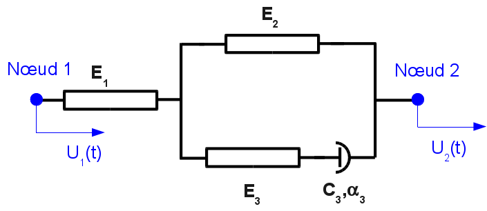
Figure 5.11.4-a: diagram of the device.
5.11.4.1. Syntax#
◊ RELATION = “DIS_VISC”
♦ GROUP_NO_1 =grno1, [group_no]
♦ GROUP_NO_2 =grno2, [group_no]
♦ /K1 =k1, [R]
/UNSUR_K1 =usk1, [R]
♦ /K2 =k2, [R]
/UNSUR_K2 =usk2, [R]
♦ /K3 =k3, [R]
/UNSUR_K3 =usk3, [R]
♦ C=c, [R]
♦ PUIS_ALPHA =/0.5 [default]
/alpha, [R]
♦ ITER_INTE_MAXI =/20 [default]
/iter [I]
♦ RESI_INTE_RELA =/1.0E-06 [default]
/resi [R]
5.11.4.2. Operands linked to the position of the device#
♦ GROUP_NO_1
♦ GROUP_NO_2
Name of the node groups in the structure between which the nonlinear device is placed. The node group should only contain one node.
When calculating, it is necessary to know the direction of the non-linear device because it only works in its axis. The distance between the two nodes must therefore be non-zero.
5.11.4.3. Behavioral operands#
Behavior DIS_VISCest a non-linear viscoelastic rheological behavior, of the extended Zener-type, making it possible to schematize the behavior of a uniaxial shock absorber, between two nodes.
For the local direction \(x\) (and only that one) of the device, five coefficients are provided. Their units should be in accordance with the unit of effort, the unit of lengths, and the unit of time of the problem:
K1: elastic stiffness of element 1 of the rheological model,
K2: elastic stiffness of element 2 of the rheological model,
K3: elastic stiffness of element 3 of the rheological model,
UNSUR_K1: elastic flexibility of element 1 of the rheological model,
UNSUR_K2: elastic flexibility of element 2 of the rheological model,
UNSUR_K3: elastic flexibility of element 3 of the rheological model,
PUIS_ALPHA: the power of the viscous behavior of the element \(\alpha\),
C: coefficient of the viscous behavior of the element.
There are conditions that must be met on the values of the coefficients in order for the tangent to always be defined:
\(\mathit{k1}\ge {10}^{-8}\) \(\mathit{usk1}\ge 0\) \(\mathit{k3}\ge {10}^{-8}\) \(\mathit{usk3}\ge 0\) \(\mathit{usk2}\ge {10}^{-8}\) \(\mathit{k2}\ge 0\) \(C\ge {10}^{-8}\) \({10}^{-8}\le \alpha \le 1\)
We therefore cannot have both \(\mathit{usk1}=0\), \(\mathit{usk3}=0\) and \(\mathit{k2}=0\) at the same time, i.e. the case of the shock absorber alone.
5.11.5. Nonlinearity: DIS_ECRO_TRAC#
Behavior DIS_ECRO_TRAC is a non-linear behavior, making it possible to schematize the behavior of a uniaxial device, along the local axis \(x\) or in the tangential plane \(\mathit{yz}\).
Note:
It’s a non-linear behavior between two nodes, so there is no finite element between the nodes concerned (just a behavioral relationship). When calculating the reduced modal base, it**may be a good idea to define an element with an elastic stiffness corresponding to the tangent to the behavior of the device*[:external:ref:`R5.03.17 <R5.03.17>`] . *
The non-linear behavior is given by a \(F=\mathit{fonction}(\mathrm{\Delta }U)\) curve:
\(\mathrm{\Delta }u\) represents the relative displacement of the 2 nodes in the local coordinate system of the element.
\(F\) represents the effort expressed in the element’s local coordinate system.
5.11.5.1. Syntax#
◊ RELATION = “DIS_ECRO_TRAC”
♦ GROUP_NO_1 =grno1, [group_no]
♦ GROUP_NO_2 =grno2, [group_no]
♦/FX =fx, [function]
/FTAN =ftan, [function]
# if function FTAN is given
♦ WORKING = | “ISOTROPIC”,
“CINEMATIC”♦ ITER_INTE_MAXI =/20 [default]
/iter [I]
♦ RESI_INTE_RELA =/1.0E-06 [default]
/resi [R]
5.11.5.2. Operands linked to the position of the device#
♦ GROUP_NO_1
♦ GROUP_NO_2
Name of the node groups in the structure between which the nonlinear device is placed. The node group should only contain one node.
When calculating, it is necessary to know the direction of the non-linear device because it only works in its axis. The distance between the two nodes must therefore be non-zero.
5.11.5.3. Behavioral operands: FX or FTAN#
The only data needed is the function describing the non-linear behavior. This function must meet the following criteria:
It is a function in the sense of code_aster: defined with the operator DEFI_FONCTION,
The interpolations on the abscissa and ordinate axes are linear,
The name of the abscissa when defining the function is DX or DTAN,
Extensions to the left and right of the function are excluded,
The function must be defined by at least 3 points,
The first point is \((\mathrm{0.0,}0.0)\) and must be given,
The function must be strictly increasing.
The derivative of the function must be less than or equal to its derivative at point \((\mathrm{0.0,0}.0)\).
Examples of the definition of the FX function:
LeSx = (0.0, 0.2, 0.3, 0.50)
LesY = (0.0, 500.0, 800.0, 900.0)
fctsy1 = DEFI_FONCTION (NOM_PARA =”DX”,
ABSCISSE = LeSx,
ORDONNEE = LeSY,
)
fctsy2 = DEFI_FONCTION (NOM_PARA =”DX”,
VALE = ( 0.0, 0.0, 0.2, 0.2, 0.2, 500.0, 0.50, 900.0 ),
)
Examples of defining function FTAN:
LeSx = (0.0, 0.2, 0.3)
LesY = (0.0, 500.0, 800.0)
fctsy1 = DEFI_FONCTION (NOM_PARA =” DTAN “,
ABSCISSE = LeSx,
ORDONNEE = LeSY,
)
fctsy2 = DEFI_FONCTION (NOM_PARA =” DTAN “,
VALE = ( 0.0, 0.0, 0.0, 0.2, 500.0, 0.3, 800.0 ),
)
The first two points of the function are used to define the elastic slope to the behavior. The x-axis and ordinate units should be consistent with those of the problem:
The unit of the abscissa must be homogeneous when moving,
The unity of function should be consistent with efforts.
5.11.5.4. Operands related to the convergence of device behavior#
♦ ITER_INTE_MAXI =/20 [default]
/iter [I]
♦ RESI_INTE_RELA =/1.0E-06 [default]
/Resi [R]
These operands have the same meaning as when used with the STAT_NON_LINE/COMPORTEMENT [U4.51.11] command.
Behavioral relationship DIS_ECRO_TRAC requires solving a nonlinear system using a 5-order Runge-Kutta method with adaptive steps. Algorithm control (number of iterations and residue) are used to test convergence and adapt the step if necessary.
5.11.6. Nonlinearity: CHOC_ELAS_TRAC#
Behavior CHOC_ELAS_TRAC is a non-linear elastic behavior, making it possible to schematize the behavior of a uniaxial device, along the local axis \(x\)
Note:
It’s a non-linear behavior between two nodes, so there is no finite element between the nodes concerned (just a behavioral relationship). When calculating the reduced modal base, it may be a good idea to define an element with an elastic stiffness corresponding to the tangent to the behavior of the device [R5.03.17] .
The non-linear elastic behavior is given by a curve \(F=\mathit{fonction}(\mathrm{\Delta }U)\):
\(\mathrm{\Delta }u\) represents the relative displacement of the 2 nodes in the local coordinate system of the element.
\(F\) represents the effort expressed in the element’s local coordinate system.
5.11.6.1. Syntax#
◊ RELATION = “CHOC_ELAS_TRAC”
♦ GROUP_NO_1 = grno1, [group_no]
♦ GROUP_NO_2 = grno2, [group_no]
♦ FX = fx, [function]

◊ DIST_1 = dist1, [R]

◊ DIST_2 = dist2, [R]
5.11.6.2. Operands GROUP_NO_1/GROUP_NO_2#
♦ GROUP_NO_1
♦ GROUP_NO_2
Name of the node groups in the structure between which the nonlinear device is placed. The node group should only contain one node.
When calculating, it is necessary to know the direction of the non-linear device because it only works in its axis.
5.11.6.3. Operands DIST_1/DIST_2#
◊ DIST_1 = dist1
Characteristic distance of surrounding material GROUP_NO_1: no1.
Operand specific to the contact between two mobile structures.
◊ DIST_2 = dist2
Characteristic distance of surrounding material GROUP_NO_2: no2.
Operand specific to the contact between two mobile structures.
Notes: DIST_1et * DIST_2 * are defined in the sense of the outgoing normals of the two solids opposite each other (DIST_1et * DIST_2sont positive because they represent the thickness of the structures studied) .
5.11.6.4. Behavioral operand: FX#
The only data needed is the function describing the non-linear behavior. This function must meet the following criteria:
It is a function in the sense of code_aster: defined with the operator DEFI_FONCTION,
The interpolations on the abscissa and ordinate axes are linear,
The name of the abscissa when defining the function is DX.
The extension of the function to the left is excluded,
The extensions to the right of the function are excluded or linear,
The function must be defined by at least 2 points,
The first point is \((\mathrm{0.0,}0.0)\) and must be given,
The function must be strictly increasing.
The x-axis and ordinate units should be consistent with those of the problem:
The unit of the abscissa must be homogeneous when moving,
The unity of function should be consistent with efforts.
5.11.7. Nonlinearity: FLAMBAGE#
◊ RELATION = “FLAMBAGE”
This relationship is used for the detection of possible buckling and for the evaluation of the residual deformation of an element during an impact between two mobile structures or between a mobile structure and a fixed wall. The reaction force during an impact taking into account buckling can be summarized by the following diagram:
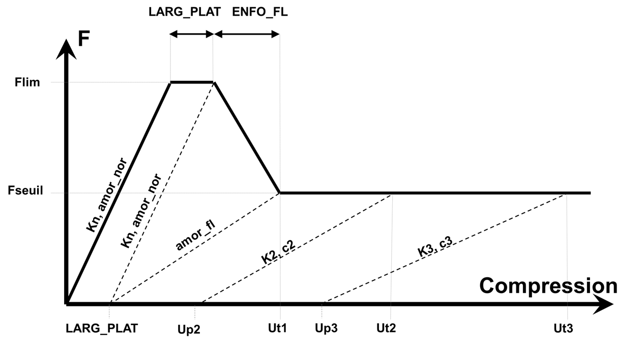
Figure 5.11.7-a: Full buckling law
Buckling is considered to occur if the reaction force \(F\) reaches the limit value \(\text{Flim}\) defined by the user. It is possible to keep the buckling force constant during compression \(\text{LARG\_PLAT}\). In this zone, the shock stiffness remains constant (\(\text{Kn}\)). Following this plateau, during buckling, the maximum force decreases progressively. The compression during buckling corresponds to user data \(\text{ENFO\_FL}\). During buckling, the stiffness decreases, but the residual deformation remains constant and equal to \(\text{LARG\_PLAT}\).
After buckling, the shock stiffness is updated based on compression and stiffness values given by the user.
The Figure shows the evolution of the force as a function of compression considering a zero shock speed, but the buckling law also takes into account the shock speed. At any moment, if the shock is detected, \(F=K(u)\times u+\mathit{Famor}(v)\), with \(u\) the compression between the two knots and \(v\) the relative speed of the knots.
\(\mathit{Famor}(v)\) depends on the maximum compression \(\mathit{Ut}\) reached during the calculation:
if \(\mathit{Ut}\le \text{LARG\_PLAT}\), then \(\mathit{Famor}(v)={\mathit{amor}}_{\mathit{nor}}\times v\)
if \(\text{LARG\_PLAT}<\mathit{Ut}\le {\mathit{Ut}}_{1}\), then \(\mathit{Famor}(v)=c\times v\), with \(c\) interpolated linearly between \({\mathit{amor}}_{\mathit{nor}}\) and \({\mathit{amor}}_{\mathit{fl}}\) according to the value of \(\mathit{Ut}\) between \(\text{LARG\_PLAT}\) and \({\mathit{Ut}}_{1}\)
if \({\mathit{Ut}}_{1}<\mathit{Ut}\le {\mathit{Ut}}_{2}\), then \(\mathit{Famor}(v)=c\times v\), with \(c\) interpolated linearly between \({\mathit{amor}}_{\mathit{fl}}\) and \({c}_{2}\) according to the value of \(\mathit{Ut}\) between \({\mathit{Ut}}_{1}\) and \({\mathit{Ut}}_{2}\)
if \({\mathit{Ut}}_{i}<\mathit{Ut}\le {\mathit{Ut}}_{(i+1)}\), then \(\mathit{Famor}(v)=c\times v\), with \(c\) interpolated linearly between \({c}_{i}\) and \({c}_{(i+1)}\) according to the value of \(\mathit{Ut}\) between \({\mathit{Ut}}_{i}\) and \({\mathit{Ut}}_{(i+1)}\)
Only operands specific to the FLAMBAGE keyword are detailed. The other keywords make it possible to define the places of shock and are identical to the operands for the DIS_CHOC relationship (see § 5.11.1).
By default, values \(\text{LARG\_PLAT}\) and \(\text{ENFO\_FL}\) are zero. The law then corresponds to the law below.
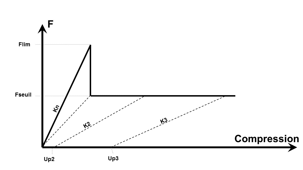
Figure 5.11.7-b: Buckling law with default values
◊ FNOR_CRIT = Movie
Limiting normal force that causes the structure to buckle.
◊ FNOR_POST_FL = Threshold
Limit normal force after buckling that causes residual deformation of the structure.
◊ AMOR_NOR =/0., [DEFAUT]
/amor_nor, [R]
Normal shock absorption value during the elastic phase and the compression plateau.
◊ ENFO_FL = /1.E-20, [DEFAUT]
/enfo_fl, [R]
Compression during buckling.
◊ LARG_PLAT = /0.0, [DEFAUT]
/large_flat, [R]
Compression during which the force remains constant and equal to Flim.
◊ DEPL_POST_FL = depl_post_fl, listr8
List of residual post-buckling compression values:depl_post_fl= [Up2, Up3,…]
◊ RIGI_POST_FL = rigi_post_fl, listr8
List of post-buckling stiffness values: rigi_post_fl= [K2, K3,…]
Lists DEPL_POST_FL and RIGI_POST_FL should be the same length.
If during the calculation, the compression exceeds the value \(\mathit{Upi}+\frac{\mathit{Fseuil}}{\mathit{Ki}}\), with \(\mathit{Upi}\) the last value specified in DEPL_POST_FL and \(\mathit{Ki}\) the last value specified in RIGI_POST_FL, an alarm is issued and the stiffness remains constant (\(\mathit{Ki}\)).
The total compression values are the sum of the residual compressions \(\mathit{Upi}\) and the elastic \(\frac{\mathit{Fseuil}}{\mathit{Ki}}\) compressions. These values should be increasing and the lowest value should be greater than \(\frac{\mathit{Flim}}{\mathit{Kn}}+\text{LARG\_PLAT}+\text{ENDO\_FL}\).
◊ AMOR_FL = amor_fl, listr8
Normal shock absorption value during the elastic phase and the compression plateau.
◊ AMOR_POST_FL = amor_post_fl, listr8
List of normal post-buckling damping values: amor_post_fl= [c2, c3,…]
Lists DEPL_POST_FL and AMOR_POST_FL should be the same length.
If during the calculation, the compression exceeds the value \(\mathit{Upi}+\frac{\mathit{Fseuil}}{\mathit{Ki}}\), with \(\mathit{Upi}\) the last value specified in the last value specified in DEPL_POST_FLet \({c}_{i}\) the last value specified in AMOR_POST_FL, the damping remains constant (\({c}_{i}\)).
◊ CRIT_AMOR=| “INCLUDED”, [DEFAULT]
| 'EXCLUDED'
The keyword CRIT_AMOR makes it possible to specify whether the buckling criterion is compared to the total shock force, or only to the part related to the shock stiffness. If CRIT_AMOR = “INCLUS”, the buckling criterion is compared to the total shock force \(K(u)\times u+\mathit{Famor}(v)\). In this case, the total shock force can never exceed the buckling criterion. If CRIT_AMOR = “EXCLUS” the viscous force is not included when comparing to the criterion. The buckling criterion is compared to the force generated by the stiffness and the \(K(u)\times u\) depression. In this case, the total shock force may be greater than the buckling criterion.
5.11.8. Nonlinearity: RELA_EFFO_DEPL#
◊ RELATION = 'RELA_EFFO_DEPL'
This relationship makes it possible to define a force-displacement or moment-rotation relationship over a given degree of freedom in the form of a non-linear curve.
5.11.8.1. Operand GROUP_NO#
♦ GROUP_NO = big
The node in the structure that the relationship is about.
5.11.8.2. Operand SOUS_STRUC#
◊ SOUS_STRUC = ss
Name of the substructure containing the node containing the GROUP_NO operand.
5.11.8.3. Operand NOM_CMP#
◊ NOM_CMP = nomcmp
The name of the node component of the structure that the relationship is about.
5.11.8.4. Operand FONCTION#
♦ FONCTION = f
Name of the nonlinear function.
The nonlinear relationship should be set to*on* \(\left]\mathrm{-}\mathrm{\infty },\mathrm{\infty }\right[\) . The nonlinear phase in post-treatments corresponds to the time range when the nonlinear relationship was non-zero.
The equilibrium equation, for a structure subject to horizontal ground acceleration \({a}_{x}\) in the \(x\) direction, and having correction terms derived from non-linearities, is written:
where \({F}_{c}\) is the corrective force due to the nonlinearity of the ground. For example, it can be defined by the following relationship (cf. test case SDND103):
with:
In the example above, under operand RELATION, we therefore impose the function:
5.11.9. Nonlinearity: RELA_EFFO_VITE#
◊ RELATION = 'RELA_EFFO_VITE'
This relationship makes it possible to define a force-speed relationship over a degree of freedom of a given node in the form of a non-linear function.
The operands GROUP_NO, SOUS_STRUC, NOM_CMP, and FONCTION have the same meaning for the RELA_EFFO_DEPL and RELA_EFFO_VITE relationships. Therefore, they are not detailed in this paragraph.
5.12. Keyword ARCHIVAGE#
◊ ARCHIVAGE
Keyword: factor that defines archiving.
5.12.1. Operand LIST_INST/INST#
◊/LIST_INST = l_arch
List of reals defining the calculation times for which the solution must be archived in the tran_gene result concept.
◊/INST
Computational moments for which the solution must be archived in the resulttran_gene concept.
5.12.2. Operand PAS_ARCH#
◊ PAS_ARCH = IPA
Integer defining the archiving periodicity of the transient calculation solution in the tran_gene result concept.
If ipa = 5 we archive every 5 calculation steps.
Regardless of the archiving option chosen, the first and last time steps and all associated fields are archived to allow possible recovery.
Note:
PAS_ARCHet LIST_INST/INSTpeuvent to both be present. In this case, the union of the times defined by these two criteria is archived.
5.12.3. Operand CRITERE#
◊ CRITERE =
Indicates how precisely the search for the moment to be archived must be done:
“RELATIF”: search interval [(1-prec).instant, (1+prec).instant]
“ABSOLU”: search interval [instant-prec, instant+prec]
The default value for the search criteria is” RELATIF “.
5.12.4. Operand PRECISION#
◊ PRECISION =/1.E-06 [DEFAUT]
/prec [R]
Indicates how precisely the search for the moment to be archived should be done.
5.13. Operand INFO#
◊ INFO = imp
Integer used to specify the printing level in the file MESSAGE.
If INFO =1, a summary of the dynamic calculation is printed with the options chosen, the matrices and the number of nonlinearities considered. The progress of the calculation is counted in increments of 5% of the total simulation time.
If INFO: 2, in addition to the information written in the case where INFO is 1, we print the progress with slices shorter than 1%. In the presence of localized nonlinearities, the following additional information is printed for each obstacle:
The number and type of the obstacle;
The name and coordinates in the global coordinate system of the shock node (shock nodes in the case of an impact between mobile structures);
The orientation, in the global frame of reference, from normal to obstacle;
The value of the spin angle;
The value of the initial game;
If mode VERI_CHOC is activated, for each shock node and for each mode, the values of the local shock stiffness and of the local flexibility rate and of the local flexibility are also printed.
5.14. Operand IMPRESSION#
◊ IMPRESSION
Keyword factor that makes it possible to print in file RESULTAT quantities that cannot be printed by a printing operator, such as local displacement, local speed, contact forces at shock nodes and the cumulative value over all modes of the modal base for projecting the rate of reconstruction of the static solution.
5.14.1. Operands TOUT/NIVEAU#
The NIVEAU keyword allows you to print one or more array (s) among “DEPL_LOC”, “VITE_LOC”, “FORC_LOC” and “TAUX_CHOC”. With TOUT = “OUI” (by default), we print the four tables.
5.14.2. Operands INST_INIT/INST_FIN#
These two keywords allow the user to filter the impressions in each loop over the time steps.
5.14.3. Operand UNITE_DIS_VISC#
◊ UNITE_DIS_VISC = unit
The results concerning the effort, the viscous and relative displacements between the two nodes, as well as the dissipation of the non-linear device can be saved in a file directly usable by the code_aster commands.
5.15. Control phase#
5.15.1. Verification on matrices#
In the case of a calculation by modal recombination, it is verified that the generalized matrices are indeed derived from a projection on a common base and with the same number of base vectors. In the case of a calculation by dynamic substructuring, it is verified that the generalized matrices actually come from the same generalized numbering.
5.15.2. Verification and advice on choosing the time step for diagrams DIFF_CENTRE, DEVOGE and NEWMARK:#
We ensure that the time step chosen verifies the stability conditions of the numerical diagram (criterion CFL):
in the case of NEWMARK, stability is always ensured but exceeding the criterion may cause a lack of precision in the result and is reported by a message; the calculation continues (at the risk of producing an inaccurate or false result).
in the case of the DIFF_CENTRE and DEVOGE schemes, if the VERI_PAS operand is equal to “OUI” (value by default), the execution is stopped, a minimum time step is proposed. If the operand VERI_PAS is equal to “NON” or if it is an adaptive schema, an alarm message is sent and the calculation continues (at the risk of producing an inaccurate or false result).
In a transient analysis without nonlinearity, care must be taken to ensure that the time step is such that:
\(\mathit{dt}<\mathrm{0,1}\mathrm{/}{f}_{n}\) for NEWMARK and DEVOGE
\(\mathit{dt}<\mathrm{0,05}\mathrm{/}{f}_{n}\) for DIFF_CENTRE
\({f}_{n}\) being the highest frequency of the modes in the modal base under consideration.
Note:
It is mentioned that with localized nonlinearities the time step chosen must sometimes be much lower than this recommended value.
5.15.3. Execution phase for adaptive schemas:#
The execution is interrupted when the time step reaches a minimum step equal to PAS_MINI.
Notes:
The s schema s ADAPT_ORDRE1 /2 (centered differences) does not accurately reproduce the natural pulsations of a system, which leads to significant calculation errors in the following two cases:
Calculation of a very large number of periods of free oscillations;
Calculation of the oscillations of a very weakly damped system ( \(\xi <{10}^{-3}\) ) excited at a resonance frequency.
In both cases, it is often necessary to increase the parameter NB_POIN_PERIODE.
The “ ADAPT_ORDRE1 “and “ ADAPT_ORDRE2 “methods can be used in substructuring.
The time step can be retrieved by the operator RECU_FONCTION, with the following syntax:
not = RECU_FONCTION (
RESU_GENE = dynamoda
NOM_CHAM = “PTEM “
…)
5.16. Taking into account fluid-structure interaction effects#
Below are the keywords specific to the calculation of the response of very weakly damped linear mechanical systems with fluidelastic couplings possibly associated with nonlinearities localized at the nodes such as shocks and frictions.
◊ BASE_ELAS_FLUI = meles
Modal base used for the calculation.
Melasflu-like concept produced by the operator CALC_FLUI_STRU [U4.66.02] which contains all the modal bases calculated for the various defined flow velocities. This keyword is mandatory for the “ITMI” method.
The transient calculation on a modal basis modified by fluidelastic coupling is carried out by taking into account the values of the added damping, due to the flow of the fluid, which are present in the melasflu concept of entry. Modal amortizations, retrieved from the base fluidelastic, replace those entered under the keyword global **** AMOR_REDUITde the operator**** DYNA_VIBRA. **
◊ NUME_VITE_FLUI = Nvitf
Flow speed used for the calculation (order number).
Allows to extract in the melasflu concept the modal base corresponding to the selected flow speed (cf. [U4.66.02]).