3. Operands

3.1. Principles

This command makes it possible to count the number of eigenvalues included in (cf. figure 3ab):

• A real axis interval (for generalized GEPs standard problems with symmetric real matrices): keyword TYPE_MODE =” DYNAMIQUE “or” MODE_FLAMB “or” GENERAL “.

• A disk of the complex plane (for all other scenarios, other GEPs and all quadratic problems QEPs): keyword TYPE_MODE =” MODE_COMPLEXE “or” GENERAL “.

This number of specific modes is plotted in the message file for each interval of the real axis or for the portion of the complex plane chosen (cf. FIG. 1). The characteristics of these areas of interest are also recalled.

---

VERIFICATION OF SPECTRE OF FREQUENCES (METHODE OF STURM)

THE NOMBRE OF FREQUENCES DANS THE BANDE N 1 OF

BORNES (0.000E+00, 1.000E+01) EST 20

---

THE NOMBRE OF FREQUENCES DANS THE BANDE N 2 OF

BORNES (1.000E+01, 2.000E+01) EST 43

…

THE NOMBRE OF FREQUENCES DANS THE BANDE N 6 OF

BORNES (5.000E+01, 6.000E+01) EST 139

---

Figure 1._ Displays in the message file of a INFO_MODE on a frequency series FREQ =( 0.,10., 20.,… ,50., 60.) for a DYNAMIQUE problem.

All these elements are stored in an sd_table (cf. figure 2ab) that can be printed (via a IMPR_TABLE) or reused (by linking with CALC_MODES). The additional cost of this operator can then become almost negligible since the global information generated is shared with other modal operators.

# TABLE_SDASTER

FREQ_MIN FREQ_MAX BORNE_MIN_EFFECT BORNE_MAX_EFFECT NB_MODE

0.00000E+00 1.00000E-02 0.00000E+00 1.00000E-02 3

1.00000E-02 5.00000E-02 1.00000E-02 5.00000E-02 3

5.00000E-02 5.50000E-02 5.00000E-02 5.50000E-02 1

5.50000E-02 6.00000E-02 5.50000E-02 6.00000E-02 0

6.00000E-02 1.00000E-01 6.00000E-02 1.00000E-01 3

# TABLE_SDASTER

CHAR_CRIT_MIN CHAR_CRIT_MAX BORNE_MIN_EFFECT BORNE_MAX_EFFECT NB_MODE

-1.00000E+06 -5.00000E+05 -1.00000E+06 -5.00000E+05 1

-5.00000E+05 0.00000E+00 -5.00000E+05 0.00000E+05 0.00000E+00 3

0.00000E+00 1.00000E+05 0.00000E+00 1.00000E+05 0

1.00000E+05 1.10000E+06 1.00000E+05 1.10000E+06 5

Figure 2ab._ Example 1 of a table generated by a INFO_MODE on a series of frequencies FREQ =( 0.,1.E-2,… ,1.E-1) for a dynamic problem. Retrieved from sdlx201a.mess. Example #2 of a table generated by a INFO_MODE on a series of critical loads CHAR_CRIT =( -1.E+6, -5.E+5,… ,1.1E+6) for a buckling*problem. Retrieved from sdls504a.mess*

Calling this operator is recommended as verification/calibration a priori of the model. It also makes it possible to define search intervals containing a reasonable number of eigenvalues (typically around forty modes) in order to optimize the costs of subsequent modal operators and to step down the precision of their results.

Typically, we recommend looking for modes in packs of about forty [3] _ . Beyond that, the consumption of time and memory is no longer optimal and the quality of the modes obtained deteriorates. It is then better to use several frequency bands (or critical loads) directly with CALC_MODES and the “BANDE” option split over several sub-bands, or by several calls to CALC_MODES [U4.52.02].

Ideally, to effectively treat a standard GEP, we propose to proceed in several steps:

• Calibrate the areas of interest by pre-calculations using only INFO_MODE (sequentially or, if possible, in parallel) on given frequency lists (resp. critical loads);

• Relaunch one or more CALC_MODES calculations with OPTION =” BANDE “based on these initial calibrations.

To save time, you can even mutualize (and it’s highly recommended!) part of the calculation cost of the initial INFO_MODE by notifying CALC_MODES of the name of the generated sd_table. This chaining can thus make the additional cost of INFO_MODE negligible and guide the modal calculation effectively.

On the intensive computing side, the INFO_MODE operator, just like CALC_MODES with the “BANDE” option divided into several sub-bands, potentially benefits from two levels of parallelism (cf. keyword NIVEAU_PARALLELISME). Hence time savings of a factor of up to 70 over a hundred processors and gains in peak memory up to a factor of 2.

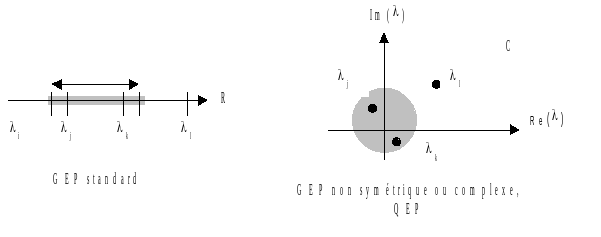
Figure 3ab._ Two distinct counting problems: in a segment of the real axis and in a finite portion of the complex plane (for the time being a disk) .

In the first case, when one seeks to count the eigenvalues strictly included in a segment of the real axis, one uses the so-called « Sturm » method, in the second case the APM method. Their theories and algorithms are detailed in the reference material [R5.01.04].

When treating standard GEPs, running this procedure generally does not require [4] _ only a factorization LDLT per mode (METHODE =” STURM “). When they are scattered throughout the complex plane, the procedure is much more expensive (METHODE =” APM “) because it generally requires hundreds of factorizations. In this case, it is therefore rather reserved for simplified problems of small sizes (less than 1000 degrees of freedom).

Note that this last method APM is still the subject of active research. Its robustness is therefore, for the moment, not guaranteed. It should be used while taking care to read the associated documentation.

3.2. Characteristics of the modal problem: operands MATR_RIGI/MATR_A//MATR_MASS/MATR_RIGI_GEOM//MATR_B/MATR_AMOR/MATR_C

The table below represents the operands to use according to the type of keyword TYPE_MODE.

TYPE_MODE
“DYNAMIQUE”	“MODE_FLAMB”	“MODE_COMPLEXE”	“GENERAL”
♦ MATR_RIGI = A	♦ MATR_RIGI = A	♦ MATR_RIGI = A	♦ MATR_A = A
♦ MATR_MASS = B	♦ MATR_RIGI_GEOM = B	♦ MATR_MASS = B	♦ MATR_B = B
Not applicable	Not applicable	◊ MATR_AMOR = C	◊ MATR_C = C

These operands make it possible to fill in matrices (assembled or generalized) [5] _ ) characterizing the modal problem. These matrices may or may not be symmetric. They are real except for matrix \(\mathrm{A}\), which can be either real or complex.

The data from \(\mathrm{A}\) and \(\mathrm{B}\) makes it possible to define the generalized modal problem (GEP) (cf. [R5.01.01]) studied

\(\mathrm{A}\mathrm{u}\mathrm{=}\lambda \mathrm{B}\mathrm{u}({\mathrm{GEP}}_{\mathrm{dynamique}})\)

In the classical case of dynamics (TYPE_MODE =” DYNAMIQUE “), \(\mathrm{A}\) is the stiffness matrix (real symmetric) and \(\mathrm{B}\) is the mass matrix (real symmetric). The eigenvalue \(\lambda\) is then linked to the natural frequency \(f\) by the formula: \(\lambda \mathrm{=}{(2\pi f)}^{2}\). It is a real positive one.

In the case of linear buckling theory (TYPE_MODE =” MODE_FLAMB “),

\(\mathrm{A}\mathrm{u}\mathrm{-}\lambda \mathrm{B}\mathrm{u}\mathrm{=}0({\mathrm{GEP}}_{\mathrm{flambement}})\)

\(\mathrm{A}\) is the stiffness matrix (real symmetric) and \(\mathrm{B}\) is the geometric rigidity matrix (real symmetric). The eigenvalue \(\lambda\) is called critical load. It is real.

As mentioned in the previous table, these matrices will be filled in, respectively, for the dynamics by MATR_RIGI/MATR_MASS and, in buckling, by MATR_RIGI/MATR_RIGI_GEOM. Only the so-called “STURM” method is legal in these two cases.

When one of the two matrices is no longer symmetric or contains complex terms (e.g. to take into account hysteretic damping), the eigenvalues are potentially complex. To deal with this problem you have to initialize TYPE_MODE to “MODE_COMPLEXE” and only the APM method is then legal.

The data from \(\mathrm{A}\) , \(\mathrm{B}\) and \(\mathrm{C}\) makes it possible to define the quadratic modal problem (QEP) (cf. [R5.01.02]) studied

\((\mathrm{A}+\lambda \mathrm{C}+{\lambda }^{2}\mathrm{B})\mathrm{u}\mathrm{=}0(\mathrm{QEP})\)

In this case, the eigenvalues are potentially complex. To deal with this problem you need to initialize TYPE_MODE to “MODE_COMPLEXE”. Often \(\mathrm{A}\) is the stiffness matrix, \(\mathrm{C}\) a matrix taking into account viscous damping and/or gyroscopic effects and \(\mathrm{B}\) the geometric rigidity matrix. As mentioned in the previous table, these matrices will be filled in by MATR_RIGI/MATR_MASS/MATR_AMOR and only the APM method is legal.

The TYPE_MODE =” GENERAL “solves an eigenvalue problem in the general case. We then make the matrices \(\mathrm{A}\) , \(\mathrm{B}\) and/or \(\mathrm{C}\) play the role we want. As mentioned in the previous table, these matrices will be filled in by MATR_A/MATR_B/MATR_C. Depending on the case, only the Sturm method (if MATR_C is not entered and if the other two matrices are symmetric real) or the APM method (all other cases) are legal.

3.3. Operand TYPE_MODE

/”MODE_FLAMB” /”MODE_COMPLEXE” /”GENERAL”

This keyword makes it possible to define the nature of the modal problem to be treated: pre-estimate the vibration frequency spectrum (classic case of “DYNAMIQUE”), do it in terms of critical loads (case of the linear buckling theory “MODE_FLAMB”) or calibrate that of a non-standard GEP or of a QEP in a portion of the complex plane (“MODE_COMPLEXE”). You can also search for the eigenvalues and the associated modes of a general matrix system (“GENERAL”). For more details, refer to the description in §3.2.

At the end of this choice, the user must specify the characteristics of his control zone:

for “DYNAMIQUE”: frequency list*via FREQ,

for “MODE_FLAMB”: list of critical loads*via CHAR_CRIT,

for “MODE_COMPLEXE”: area of the complex plane*via TYPE/RAYON/CENTRE_CONTOUR,

• for “GENERAL”: depending on the case, either we proceed as for “MODE_FLAMB” (if MATR_Cn is not specified and if the other two matrices are symmetric real), or as for “MODE_COMPLEXE” (all other cases).

3.4. Operand FREQ

List of frequencies (in Hertz) defining the intervals you want to calibrate \(\text{l\_f}\mathrm{=}{({f}_{i})}_{i}\) (the number of frequencies in this list is denoted nb_freq). We then look for the number of eigenvalues in sub-bands \(\mathrm{[}{\lambda }_{i},{\lambda }_{\text{i+1}}\mathrm{]}\) with \({\lambda }_{\text{*}}\mathrm{=}{(2\pi {f}_{\text{*}})}^{2}\). This list must include at least two values. These values must be arranged in strictly ascending order and all are positive.

This keyword should be used if TYPE_MODE =” DYNAMIQUE “. Only the counting method of type STURM is then legal.

Notes:

• Each frequency is treated only once: as the lower bound of the first sub-band for the first in the list, as the upper bound of the following sub-bands for the other frequencies. In particular, if this frequency is considered too close to an eigenvalue, it is offset (possibly several times cf. parameters PREC_SHIFT/NMAX_ITER_SHIFT etc). This « shift » shift is always carried out towards the outside of the sub-band in question.

• If the shift in the lower bound makes it bigger than the upper bound, the process stops in ERREUR_FATALE .

• This lag mode makes subsequent re-uses of this sd_table by one or more CALC_MODES more robust and consistent. In particular, sub-band overlaps that could occur up to V10 are avoided.

The initial boundaries of each of these sub-bands*are saved in the fields*FREQ_MIN/MAX*of each row of the table produced (cf. figure 2a). For each of these pairs, we mention the limits actually used by the Sturm test (i.e. after any differences), *BORNE_MIN/MAX_EFFECT, as well as the number of modes found: NB_MODE . *

3.5. Operands CHAR_CRIT

List of critical loads defining the intervals you want to calibrate \(\text{l\_c}\mathrm{=}{({\lambda }_{i})}_{i}\) (the number of critical loads in this list is denoted by nb_mode_flamb). We then look for the number of eigenvalues in sub-bands \(\mathrm{[}{\lambda }_{i},{\lambda }_{\text{i+1}}\mathrm{]}\). This list must include at least two values. These values should be arranged in strictly ascending order. They must be of a real type.

This keyword should be used if TYPE_MODE =” MODE_FLAMB “or if TYPE_MODE =” GENERAL “(if MATR_Cn is not specified and if the other two matrices are real symmetric). Only the STURMest counting method is legal.

Notes:

• Each critical load is treated only once: as the lower bound of the first sub-band for the first in the list, as the upper bound of the following sub-bands for the other frequencies. In particular, if this load is considered too close to an eigenvalue, it is offset (possibly several times cf. parameters PREC_SHIFT/NMAX_ITER_SHIFT etc). This « shift » shift is always carried out towards the outside of the sub-band in question.

• If the shift in the lower bound makes it bigger than the upper bound, the process stops in ERREUR_FATALE .

• This lag mode makes subsequent re-uses of the sd_table by one or more CALC_MODES more robust and consistent. In particular, sub-band overlaps that could occur up to V10 are avoided.

The initial boundaries of each of these sub-bands*are saved in the fields*CHAR_CRIT_MIN/MAX*of each row of the table produced (cf. figure 2b). For each of these pairs, we mention the limits actually used by the Sturm test (i.e. after any differences), *BORNE_MIN/MAX_EFFECT, as well as the number of modes found: NB_MODE . *

3.6. Operands TYPE/RAYON/CENTRE_CONTOUR

If TYPE_MODE =” MODE_COMPLEXE “or if TYPE_MODE =” GENERAL” (if MATR_C is specified or/and if one of the matrices is not symmetric or complex)

♦ RAYON_CONTOUR = radius [R] ◊ CENTRE_CONTOUR =/center [C] /0.0+0.0j [DEFAUT]

These keywords define the type of contour within which the eigenvalues and its characteristics are sought. For the moment we can only choose a “CERCLE” outline (which therefore delimits the control disk). We mention its center (a complex number) and its radius (a positive real).

Notes:

• Strictly speaking, this radius must be greater than the « modal zero ». That is, greater than the value below which we consider that an eigenvalue is zero or that two eigenvalues are confounded if we talk about their difference.

• Contrary to the values of FREQ, the units here are not in frequency, but in pulsation if we make the analogy with the problem DYNAMIQUE. As with a TYPE_MODE =” MODE_FLAMB “, the unity of the outline characteristics does not undergo any transformation. This allows method APM to deal with all types of issues.

• The table produced with the option TYPE_MODE =” MODE_COMPLEXE “contains, in addition to the number of eigenvalues ( NB_MODE ), three real ones to describe the search criteria for the APM method. The first two are CENTRE_R and CENTRE_I, the real and imaginary parts of the complex number that corresponds to the center of the search disk. The third parameter, RAYON, is the radius (strictly positive real>1.d-2) of the disk.

3.7. Keyword factor COMPTAGE

Once the type of control zone (segment or disk) has been defined, it remains to fix the counting method and its parameters.

/”STURM”, /”APM”.

If you treat a “DYNAMIQUE” or “MODE_FLAMB” problem, only the “STURM” and “AUTO” methods are allowed.

The same goes for “MODE_COMPLEXE” and “APM”/”AUTO”.

In the case of “GENERAL”, all three methods are available and the value “AUTO” then makes perfect sense! It chooses for the user between STURM and APM according to the characteristics of the modal problem:

• Or it’s a standard GEP (two real symmetric matrices): STURM method.

• In all other cases (atypical GEP with a non-symmetric and/or complex matrix or QEP): method APM.

If you leave the 'AUTO' mode set by default, the operator automatically chooses the method according to the type of study chosen. This value has been deliberately left, even in cases where there is only one alternative, to facilitate ergonomics.


If METHODE is wrong, an alarm appears and the operator automatically chooses the most appropriate method or stops at ERREUR_FATALE, depending on the situation.

Note:

• You can use the method APMpour to count the modes of a standard GEP by asking TYPE_MODE =” MODE_COMPLEXE “. This makes it possible to compare and validate the two counting methods (cf. test case SDLL123a) .

# If TYPE_MODE =' DYNAMIQUE '

◊ SEUIL_FREQ =/f_threshold [R] /0.01 [DEFAUT] ◊ PREC_SHIFT =/p_shift [R] /0.05 [DEFAUT] ◊ NMAX_ITER_SHIFT =/n_shift [I] /3 [DEFAUT]

# If TYPE_MODE =” MODE_FLAMB “or” GENERAL “(if MATR_C is not specified and if the other two matrices are symmetric real)

◊ SEUIL_CHAR_CRIT =/c_threshold [R] /0.01 [DEFAUT] ◊ PREC_SHIFT =/p_shift [R] /0.05 [DEFAUT] ◊ NMAX_ITER_SHIFT =/n_shift [I] /3 [DEFAUT]

These parameters are only used by the STURM method.

The SEUIL_ * parameters are used to define the « modal zero », i.e. the value below which the eigenvalue is considered to be zero. If we are in dynamics, we transform this value into pulsation.

\(\mathit{omecor}\mathrm{=}{(2\pi \text{f\_seuil})}^{2}\)

While in buckling we keep it as it is

\(\mathit{omecor}\mathrm{=}\text{c\_seuil}\).

The other parameters, PREC_SHIFT and NMAX_ITER_SHIFT, are linked to the algorithm for offsetting the limits of the interval (cf. [R5.01.04] §3.2) when we notice that they are very close to an eigenvalue. Roughly these boundaries \({f}_{\mathrm{min}}\) (or \({\lambda }_{\mathrm{min}}\) in buckling) or \({f}_{\mathrm{max}}\) (resp. \({\lambda }_{\mathit{max}}\)) are then offset to the outside of the p_shift% segment. If the dynamic matrix thus reconstructed is still considered « numerically singular », we re-shift again after having issued a ALARME. We try this n_shift shift times.

\({{\lambda }^{\text{-}}}_{\mathit{min}}\mathrm{=}{\lambda }_{\mathit{min}}\text{-}\mathit{max}(\mathit{omecor}{\mathrm{,2}}^{(i\mathrm{-}1)}\text{x}{p}_{\mathit{shift}}\text{x}∣({\lambda }_{\mathit{min}})∣)\) (2nd attempt)

\({{\lambda }^{\text{-}}}_{\mathit{max}}\mathrm{=}{\lambda }_{\mathit{max}}\text{+}\mathit{max}(\mathit{omecor}{\mathrm{,2}}^{(i\mathrm{-}1)}\text{x}{p}_{\mathit{shift}}\text{x}∣({\lambda }_{\mathit{max}})∣)\) (2nd attempt)

In fact, in dynamics as in buckling, the lag operates in the same way. Strictly speaking, in dynamics, it is therefore not the frequencies that are offset, but the pulsations.

Another precision, the lag is in fact, for the sake of efficiency, dichotomous: p_shift% the first time, 2xp_shift% the second time etc. This process should make it possible to quickly move away from the « zone of singularity » at a lower cost. On the other hand, the values of these parameters should not be increased too much, because due to differences, the resulting limits may turn out to be very different from the initial limits.

In addition, to remain consistent with the « modal zero » (noted here omecor):

• We do not shift by a value less than this minimum (hence the max in the formulas above),

If from the start, the gauged limit is less than this « zero » :math:`∣{lambda }_{text{}}∣<mathit{omecor}` (in absolute value) we set it to more or less this value (depending on whether this limit is positive or negative). Any time lag is then no longer allowed.

Notes:

• A bound in the range \(\sigma\) is close to an eigenvalue, when the factorization LDLT of the dynamic matrix associated with this boundary (for example that of a GEP is write \(\mathrm{Q}(\sigma )\mathrm{:}\mathrm{=}\mathrm{A}\mathrm{-}\sigma \mathrm{B}\) ), leads to a decimal loss of more than NPRECdigits (value set under the keyword SOLVEUR) .By playing on the value of this parameter (NPREC =7, 8). or 9), it is then possible to avoid the expensive refactorizations that these differences involve when this numerical singularity is not very pronounced.

• Similarly, by playing on the numerical parameters of linear solvers (for example: METHODE, RENUM, PRETRAITEMENTS …), we can also influence this singularity criterion.

# If TYPE_MODE =' MODE_COMPLEXE 'or' GENERAL '(if MATR_C is specified or/and if one of the other two matrices is not symmetric or complex)

◊ NBPOINT_CONTOUR =/nb_point [I] /40 [DEFAUT] ◊ NMAX_ITER_CONTOUR =/n_outline [I] /3 [DEFAUT]

These parameters are only used by the APM method.

The previous two parameters, NB_POINT_CONTOUR and NMAX_ITER_CONTOUR, are only used with the APM method. They are crucial for its robustness and they size its calculation time (a calculation with nb_point=80 will last longer than a calculation with nb_point=40).

The value nb_point gives the number of discretization points that are positioned along the contour. This discretization must be fine enough to "capture" all the spectral information. Ideally, this value should be set to at least six times the number of modes you expect to find in the circle. If you have no idea what this number is, you should set it to a value that is not too low: for example, 40 or 60.

Note:

• Attention, if this figure is too big (for example 1000), depending on the size of the problem, as it involves as many factorizations LDLT, the calculation can be very long!

The implemented algorithm APM will only converge when 3 successive evaluations of the number of eigenvalues provide the same result. The difference between these three evaluations lies only in the degree of discretization of the outline. We start by discretizing with :math:`{k}_{\mathrm{-}}\mathrm{=}\text{nb\_point}\mathrm{/}2`, then with :math:`k\mathrm{=}\text{nb\_point}` and finally with :math:`{k}_{+}\mathrm{=}2\text{nb\_point}`. If these three levels of contour discretization produce an estimate of the number of identical eigenvalues, the algorithm is considered to be converged. Its result is then this whole number.

Otherwise, these three levels of discretization are doubled according to the following permutation:

:math:`{k}_{\mathrm{-}}\leftarrow k`, :math:`k\leftarrow {k}_{+}`, and :math:`{k}_{+}\leftarrow 2{k}_{+}`

[6] _ . If they are the same, convergence is reached, otherwise we continue. This dichotomous heuristic is repeated a maximum of n_contour times.

If this process has not converged or if its result is inconsistent (strictly negative integer), we stop at ERREUR_FATALE.

3.8. Operand INFO

/2

Indicates the print level in file MESSAGE.

1: Impression of the result (and the main steps of the algorithm if APM).

2: More detailed impression rather for developers.

3.9. Operand TITRE

The title that will be given to the table produced.

3.10. Keyword factor SOLVEUR

◊ SOLVEUR =_F (),


We have access to all the parameters of the direct linear solvers (METHODE =' LDLT '/' MULT_FRONT '/' MUMPS ') except those explicitly linked to the final descent-ascent step. This restriction only concerns the following two parameters of the MUMPS solver: POSTTRAITEMENTS and RESI_RELA.

At the same time, we particularly recommend configuring [7] _ METHODE =” MUMPS “and RENUM =” QAMD “.

For more details on solvers, you can consult the document [:ref:`U4.50.01 <U4.50.01>`].

3.11. Operand NIVEAU_PARALLELISME

◊ NIVEAU_PARALLELISME =/'COMPLET' [DEFAUT]

/”PARTIEL”

When treating problems of medium or large size (> 0.5M degrees of freedom) and/or when looking for a good part of their spectrum (> 50 modes), the use of parallelism provides significant gains in time and memory. And this, with functional behavior and accuracy of results that are unchanged compared to the sequential mode.

The natural division of calculation INFO_MODE into independent nb_sbands (number of sub-bands=nb_freq-1 or nb_mode_flamb-1) provides a very efficient first level of parallelism (in time). It does not impact memory consumption [8] _ .

On the other hand, since most of the calculation cost is due to the numerical factorization phase [9] _ of the linear solver, if we parallelize this step via MUMPS (METHODE =” MUMPS “), we add significant gains in time and memory. It is a second level of parallelism that can be activated.

With the default value for this keyword (NIVEAU_PARALLELISME =” COMPLET “), when the calculation is parallel, the two levels of parallelism are combined. As the second (that of the linear solver) is less efficient than the first, it is only triggered if the number of processors allows it (nb_proc>nb_sband) and only if the selected linear solver supports parallelism MPI (SOLVEUR =_F (=_F (METHODE =” MUMPS “)).

If you select the other value of the keyword (NIVEAU_PARALLELISME =” PARTIEL “), you only benefit from the parallelism of the linear solver (the second level). This may be useful for testing methods or for focusing the gains on reducing the memory peak (after having tried the other lever arms proposed in the SOLVEUR keyword).

For more information on the implementation of parallelism, refer to the documentation [U2.08.06] or to the dedicated paragraph of the documentation [U2.06.01].

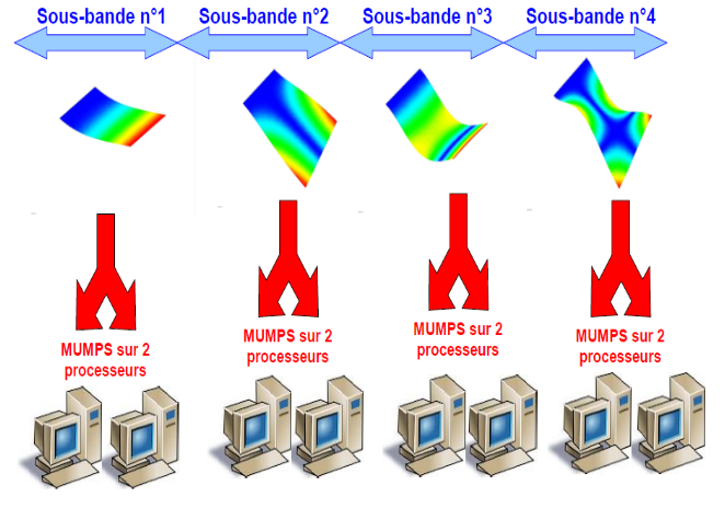
Figure 3.11-1. Example of distribution of d “INFO_MODE calculations on 8 processors with a division into 4 frequency sub-bands.

Thus, by activating only the first level of parallelism, a calculation divided into nb_sband and parallelized on nb_proc=nb_sband can save time at least one factor nb_sband/2 (without additional memory costs and without loss of precision).

If we distribute the calculation over more processors (nb_proc>nb_sband) using the solver MUMPS (thus adding the 2nd level), the time savings will be improved by a factor close to 2 for each 2* nb_sband additional processors [10] _ . And this, with memory gains of up to a factor of 2 [11] _ .

In order to maintain the efficiency of parallel calculations, we recommend:

• With “COMPLET”, select a number of processors that is a multiple of the number of sub-bands. Typically 2, 4, or 8. This limits load imbalances.

• With “PARTIEL”, reserve at least 105 degrees of freedom per processor in order to sufficiently power the MUMPS linear solver.

The functional rules are as follows, noting nb_proc the number of processors set (Astk’s option/mpi_nbCPU tab) and nb_sband the number of non-empty sub-bands:

• With NIVEAU_PARALLELISME =” COMPLET “(default): very big gain in time/improvement of the memory peak RAM.

Figure 3.11-2. Scope of use with NIVEAU_PARALLELISME =” COMPLET “.

• With NIVEAU_PARALLELISME =” PARTIEL “: moderate gain in time/significant gain on the memory peak RAM.

nb_proc

Figure 3.11-3. Scope of use with NIVEAU_PARALLELISME =” PARTIEL “ .

[1]

In sequential mode. With CALC_MODES option “BANDE” split across several parallel sub-bands, you can get a calculation more quickly by only taking about twenty modes.

[2]

Unless the value is close to an eigenmode, in which case it is « offset » (cf. keyword NMAX_ITER_SHIFT) to limit certain numerical instabilities.

[3]

This concept of a generalized matrix has nothing to do with that of a generalized modal problem!

[4]

Of course, to save computation time, we only reassess for the new discretization, the finest.

[5]

In order to minimize the time cost of the (sequential) analysis phase of MUMPS. However, this configuration is done at the expense of memory consumption. But this additional cost is quickly offset by the distribution of data on the processors that parallelism implies.

[6]

This is the case for CALC_MODES with OPTION =” BANDE “cut across several parallel sub-bands.

[7]

Stage of the linear solver that gets the most out of parallelism.

[8]

On sufficiently large problems (N>0.5M), the parallel efficiency of the factorization phase of MUMPS is often close to 0.5 (especially with a frustrating renumber type “QAMD” cf. §3.10).

[9]

In INFO_MODE, the memory consumption of MUMPS is particularly optimized: the operation in- CORE does not consume more memory than the OUT -OF- CORE (gain x3). This behavior is adapted for this operator. The gains that parallelism can give him are therefore proportionally less significant.