7. Piloting#

Piloting is sometimes known as the continuation method.

◇ PILOTAGE = _F (
        ◆ TYPE =/"ANA_LIM ",
                 /"DDL_IMPO ",
                 /"DEFORMATION ",
                 /"LONG_ARC ",
                 /"PRED_ELAS ",
                 /"SAUT_IMPO ",
                 /"SAUT_LONG_ARC ",
        ◇ COEF_MULT = float (default: 1.0),
        ◇ EVOL_PARA =/"CROISSANT ",
                      /"DECROISSANT ",
                      /"SANS" (by default),
        ◇ ETA_PILO_MAX = float,
        ◇ ETA_PILO_MIN = float,
        ◇ ETA_PILO_R_MAX = float,
        ◇ ETA_PILO_R_MIN = float,
        ◇ PROJ_BORNES =/"NON ",
                        /"OUI" (by default),
        # If: equal_to (" TYPE ", 'LONG_ARC') or equal_to (" TYPE ", 'SAUT_LONG_ARC')
            ◇ SELECTION =/"ANGL_INCR_DEPL ",
                          /"MIXTE ",
                          /"NORM_INCR_DEPL" (by default),
                          /"RESIDU ",
        # If: not equal_to (" TYPE ", 'LONG_ARC') and not equal_to (" TYPE ", 'SAUT_LONG_ARC')
            ◇ SELECTION =/"MIXTE ",
                          /"NORM_INCR_DEPL" (by default),
                          /"RESIDU ",
        ◇/TOUT = "OUI" (or not specified),
          /GROUP_MA = grma,
        ◇ FISSURE = fiss_xfem,
        ◇/NOEUD = no,
          /GROUP_NO = grno,
        ◇ NOM_CMP = text,
        ◇ DIRE_PILO = text,
    ),

7.1. General principles#

When the \(\eta\) intensity of a portion of the load is not known a first (so-called reference loading defined in [AFFE_CHAR_MECA] with load type FIXE_PILO), the keyword PILOTAGE makes it possible to control this load through a node (or group of nodes) on which you can impose different driving modes (keyword TYPE).

Notes:

With FIXE_PILO, you cannot use the FONC_MULT keyword for reference loading.
When the reference load is set by [AFFE_CHAR_MECA_F], this loading can be a function of space variables but not of time. Likewise, the changes resulting from control variables (such as temperature) that depend on time cannot be used with the pilot.
Piloting with contact is prohibited (except in the case of contact XFEM).
It is not possible to pilot with PREDICTION =” DEPL_CALCULE “or PREDICTION =” EXTRAPOLE “

7.2. The types of piloting#

The type of piloting carried out is given by the keyword TYPE. Seven driving modes are available (Confer [R5.03.80] for more details).

7.2.1. Piloting for trips#

The control for the movements will control the intensity of the load to control a displacement or equivalent.

The TYPE =” DDL_IMPO “allows you to impose a given value for the displacement increment (a single component \(i\) possible) into a single node (or a group of nodes comprising only one single node) given by the keywords NOEUD or GROUP_NO. At each time increment, we look for the amplitude \(\eta\) of the reference load that will satisfy the relationship Next incremental

\[C \, \Delta {u}_{i} (\text{noeud}) = \Delta t\]

The TYPE =” LONG_ARC “makes it possible to control the intensity \(\eta\) of the reference load by the length (curvilinear abscissa) of the response when moving a group of nodes (to be used by example when you want to control the buckling of a test piece). The following relationship is verified:

\[C \, \parallel \Delta u\parallel =\Delta t\]

with \(\parallel (\Delta u)\parallel =(\sqrt{\sum_{n}\sum _{c}({\Delta u}_{n,c}^{2})})\)

where \(n\) are the steering nodes and \(c\) are the components of moving the nodes considered. Even if the control node group is reduced to a single node, you still have to use GROUP_NO.

For both types, \(C\) is given by the COEF_MULT keyword and NOM_CMP gives the name of the component (corresponding to the degree of freedom \(i\)) used for piloting (“DX” for example).

7.2.2. Control for cracks#

The TYPE =” SAUT_IMPO “uses the principle of TYPE =” DDL_IMPO” but to control the jump increment of displacement between the lips of a crack X- FEM. Only one \(i\) direction is possible, but it can be defined on a local basis (normal or tangent to the crack). We control the average of this jump increment over a set of intersection points. \({P}_{a}\) of the interface with the \(a\) edges of the mesh. This set describes all the crack if GROUP_NO is not filled in (behavior by default), and only a part if he is. Attention, this type of control can only be used in modeling X- FEM.

\[C \, \frac{1}{N}\sum _{a=1}^{N}〚\Delta {u}_{i}〛({P}_{a})=\Delta t\]

The TYPE =” SAUT_LONG_ARC “uses the principle of LONG_ARC but to control the increment norm of the displacement jump between the lips of a crack X- FEM. We control this standard on average. on a set of intersection points \({P}_{a}\) of the interface with the edges \(a\) mesh. This set describes the entire crack if GROUP_NO is not specified (behavior) by default), and only a portion if it is.

\[C \, \parallel \stackrel{ˉ}{〚\Delta u〛}\parallel =\Delta t\]

with \(\parallel \stackrel{ˉ}{〚\Delta u〛}\parallel =\sqrt{\frac{1}{N}\sum _{c}\sum _{a=1}^{N}{(〚\Delta {u}_{c}〛({P}_{a}))}^{2}}\) where \(c\) are the components of displacement. Even if the control node group is small with a single node, you still have to use GROUP_NO.

\(C\) is given by the COEF_MULT keyword.

The definition of the group is subtle since in modeling X- FEM we do not control values on nodes but at points of intersection between the edges of the mesh and the crack. Hereinafter, the term « edges » simply refers to intersected edges. The algorithm starts by building a set of independent edges that covers the entire crack. By default, it pilot on all these edges. The GROUP_NO keyword allows the user to restrict this together, each node entered then corresponding to the end of an edge that we want pilot. Let us then point out the following rules:

if two nodes are the respective ends of two non-independent edges, only one will be retained see Piloting for cracks with GROUP_NO not specified
if a node is the end of several edges, the first edge is arbitrarily selected encountered by the algorithm, see Nodes, endpoints of non-independent edges
if two nodes are at the end of the same crack an error will be returned. In a way In general, it is advisable that all the nodes entered be on the same side of the crack, See Error for nodes connected to the same edge
if a node does not correspond to any edge, an error is returned, See Error for node not connected to an intersected edge

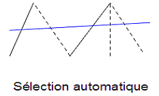
Fig. 7.1 Piloting for cracks with GROUP_NO not specified#

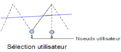
Fig. 7.2 Nodes, endpoints of non-independent edges#

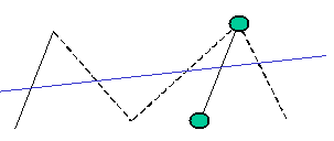
_images/100000000000012F00000080E8F924C1FD076D0E.png — Fig. 7.3 Error for nodes connected to the same edge#

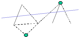
Fig. 7.4 Error for node not connected to an intersected edge#

DIRE_PILO gives the name of the \(i\) direction in which we control the movement jump. Possible values are: “DX”, “DY”, “DZ”, “DNOR” for normal to the crack, “DTAN” for the first tangent (vector product of the normal with \(X\)), “DTAN2” for the second tangent.

FISSURE gives the name of the crack XFEM on which piloting is applied.

7.2.3. Management for limit analysis#

Control TYPE =” ANA_LIM “is specific to the calculation of limit load (law NORTON_HOFF) by approach kinematics (see [ref: R7.07.01 <R7.07.01>] for more details). If \(F\) refers to controlled assembled load (indicated by TYPE_CHARGE =” FIXE_PILO “), then the pilot function is simply written:

\[P(u)=F \cdot u = 1\]

Except for limit load calculation, this feature is not of interest a priori. For this control mode, no other key word needs to be specified.

7.2.4. Management for softening behaviors#

Using softening laws of behavior can lead to brutal snap-backs that make the calculation process difficult. The following two control modes remedy this: (Cf. [R5.03.80] for more details).

Piloting TYPE =” DEFORMATION “ensures that at least one Gauss point in the structure sees its deformation evolves monotonously. We check the relationship:

\[C \,\underset{\mathrm{Pg}}{\mathrm{max}} \left( \frac{\dot{\varepsilon}}{\parallel \dot{\varepsilon }\parallel } \cdot \Delta \varepsilon \right) =\Delta t\]

This control mode is valid for all laws of behavior, including in large deformations SIMO_MIEHE.

The control TYPE =” PRED_ELAS “ensures that at least one Gauss point of the structure leaves the threshold of linearized elasticity \({f}_{\text{pred-elas}}\) by a quantity \(\frac{\Delta t}{C}\).

We check the relationship:

\[C \, \underset{\mathrm{Pg}}{\mathrm{max}} \left( {f}_{\mathrm{PRED\_ELAS}} \right) =\Delta t\]

This driving mode is only valid for laws ENDO_SCALAIRE (with the non-local version), ENDO_FISS_EXP (non-local only), ENDO_ISOT_BETON and ENDO_ORTH_BETON (with the local version) and the non-local version), BARENBLATT, BETON_DOUBLE_DP, CZM_EXP (with discontinuous elements) internal *_ ELDI), CZM_OUV_MIX and CZM_TAC_MIX (interface elements*_ INTERFACE), CZM_EXP_REG (joint elements *_ JOINT or modeling X- FEM) and CZM_LIN_REG (joint elements).

\(C\) is given by the COEF_MULT keyword but setting this parameter is difficult to Define at first try because the notion of criterion output \(\frac{\Delta t}{C}\) is not not intuitive and varies according to the laws of behavior. For laws ENDO_SCALAIRE, ENDO_FISS_EXP and ENDO_ISOT_BETON, a different version of the definition of \(\frac{\Delta t}{C}\) is used, where this parameter is linked to the increment damage (see [R7.01.04]).

When you want to use these driving modes, it is essential to do a first calculation without the PILOTAGE keyword to start the problem and get an initial state \({\varepsilon }^{\text{-}}\) different from zero (otherwise division by zero for piloting) by deformation increment). After a restart, starting from this initial non-zero state, is carried out. and we use piloting.

Solving the two previous equations makes it possible to obtain the unknown loading intensity. In some cases, solving these equations can lead to multiple solutions for the intensity. We then always choose the solution that is closest to \({\varepsilon }^{\text{-}}\). That is why, when you want to impose a loading Alternately, each time the sign of the load changes, you must perform a first calculation without the PILOTAGE keyword in order to obtain an initial state \({\varepsilon }^{\text{-}}\) traction or compression. A second calculation is then carried out on the basis of the previous initial state with the keyword PILOTAGE.

These two types of control are not available for structural elements.

We give the cells or groups of cells used to control the calculation by the keywords GROUP_MA, MAILLE, or TOUT. Interesting to alleviate the resolution of the equations of these modes of piloting.

7.3. Terminal control#

These keywords ETA_PILO_R_MAX and ETA_PILO_R_MIN define the search interval steering values. At each Newton’s iteration, all the driving values apart of \([\eta^{R}_{min}, \eta^{R}_{max}]\) are ignored. This can lead to « pilot failure » if this interval is too restrictive.

If you don’t specify values, it’s \(\eta^{R}_{min}=-\infty\) and \(\eta^{R}_{max}=+\infty\).

One possible use of this interval is as follows. For example, you want to pilot a pressure imposed on the structure and it is expected to maintain this positive pressure. By fixing \(\eta^{R}_{min}=-0\), this makes it possible to impose positive management values.

The keywords ETA_PILO_MAX and ETA_PILO_MIN are used to specify the range of values of desired piloting. It is used to properly stop the calculation when ETA_PILOTAGE reaches the limits of this interval.

This interval should be more restrictive than the search interval defined earlier, because this The latter is applied in all cases. The operating principle is as follows: at convergence of Newton’s iterations, if one of the limits has been reached, the calculation stops.

One possible use of this interval is as follows. In the case of the presence of a snap-back, by setting \(\eta_{min}\) to a low value, this allows you to stop the calculation before a complete tear/damage to the sample and thus avoid discrepancy at the last step of time.

The other possible use is that of \(\eta_{max}\) as a maximum load limit.

With the ENDO_ISOT_BETON law, these two keywords are mandatory, as they are used to fix the control terminals at the elementary level.

If interval \([\eta_{min}, \eta_{max}]\) is exceeded, the user can specify if he wants to project the steering value to \([\eta_{min}, \eta_{max}]\) with PROJ_BORNES =” OUI “.

With PROJ_BORNE =” OUI “, the projection will be performed (if \(\eta>\eta_{max}\) then \(\eta=\eta_{max}\); if \(\etaw\eta_{min}\) then \(\eta=\eta_{min}\)), which allows, in case of convergence to stop the calculation precisely on \(\eta_{min}\) or \(\eta_{max}\).

With PROJ_BORNE =” NON “, you don’t change the eta values, even if during the iterations of Newton the latter has a value greater than \(\eta_{max}\) or less than \(\eta_{min}\). On the other hand, the calculation is stopped, if at convergence \(\eta\) exceeds the bollards.

A possible use of the interval \([\eta_{min}, \eta_{max}]\) with the option PROJ_BORNE =” OUI “is next. For example, we want to compare several calculations for a softening model, which are piloted while on the move. These control parameters make it possible to stop the calculations at same load when the structure is sufficiently softened. This strategy makes the comparison easier, thanks to the control of the last pilot point.

It is strongly recommended to use the option PROJ_BORNE =” OUI “when setting up test cases involving load control. This in fact makes it possible to stop the calculation in specific points where values are tested, which improves the robustness of the test and facilitates its maintenance. An example of this data setting is proposed in the ssnop133a and ssnop133d tests.

With PROJ_BORNE =” NON “we can in some cases unblock the calculations, which otherwise wouldn’t do not converge with the overly restrictive conditions imposed via interval \([\eta^{R}_{min}, \eta^{R}_{max}]\). Or do we pilot a pressure imposed on the structure and it is expected to maintain this positive pressure. By fixing \(\eta^{R}_{min}=0\), the calculation stops when the pilot fails. On the other hand, by imposing \(\eta^{R}_{min}\) slightly negative, we de facto authorize the passage through a « non-physical » state during Newton iterations, which facilitates the convergence. The converged state in this case may as well be physical (positive pressure) or non-physical. It is the value of \(\eta^{R}_{min}=0\), which will govern the behavior in case of convergence off limits. This strategy makes it possible to maintain only positive management values, if finds at least one positive control value.

7.4. Multiple solution control#

The SELECTION keyword allows you to select the method for choosing the steering value in the case where several solutions are provided by the control resolution.

SELECTION =” NORM_INCR_DEPL “allows you to select the control value by the lowest standard of the displacement increment over the time step in question.

SELECTION =” ANGL_INCR_DEPL “allows you to select the control value by the smallest angle between the displacement obtained for the current time step and the displacement obtained for the time step previous time. This choice is only available with TYPE = LONG_ARC.

SELECTION =” RESIDU “allows you to select the control value leading to the smallest residue.

SELECTION =” MIXTE “allows you to select the control value based on several strategies. First, let’s start with the NORM_INCR_DEPL strategy above. If the results of the objective function (the norm of the displacement increment) are too close, we switch for this iteration on the RESIDU strategy. Again, if the residues are too close, we Go back to strategy NORM_INCR_DEPL and we examine whether the RESI_GLOB_MAXI residue list of the country Current weather has cycles. If this is the case, it is the worst solution to NORM_INCR_DEPL which is chosen for this iteration. If not, we simply choose the best of both, even if they are not sufficiently contrasting.

Note:

If you reuse the calculation with the keyword SELECTION =” ANGL_INCR_DEPL “, it is important to keep in mind that this criterion requires the previous two steps of time. Care must therefore be taken to archive the results of the previous calculation correctly. at the risk of obtaining false results. An alarm alerts the user in this situation.

The EVOL_PARA keyword makes it possible to impose the growth or decrease of the control parameter.