3. Principles#

This command makes it possible to describe areas subject to conditions of unilateral contact with or without friction. The description is at two levels:

Global parameters such as the choice of formulation or the control parameters of the non-linear resolution algorithm (fixed point or Newton loops, specific parameters for the solver);
Local settings specific to each contact area.

The concept from DEFI_CONTACT is then entered as a parameter in the simple keyword CONTACT of the operators STAT_NON_LINE [U4.51.03] and DYNA_NON_LINE [U4.53.01]. Each zone includes two surfaces that can come into contact, which are described by the data of the groups of cells that constitute them. For parallelism, we recommend using the centralized partitioning method if you use the discrete formulation and/or if you use DYNA_NON_LINE (because of the time patterns).

The sets of cells that are potentially in contact are skin elements: surface and linear in dimension 3 (QUAD9, QUAD8,, QUAD4, TRIA7, TRIA6, TRIA3, SEG3, SEG2), linear and point in dimension 2 (SEG3, SEG2 and POI1).

In dimension 2, POI1 meshes must be on the slave surface. They cannot be used with the CONTINUE formulation.

In dimension 3, SEG2ou SEG3doivent meshes must be on the slave surface. This implies that the definition of a contact between two beam elements is not possible in 3D.

Attention:

For the formulation DISCRETE, in dimension 3, the treatment of contact with quadratic edge meshes of type QUAD8 requires linking the middle nodes to the vertex nodes in order to have correct results. This operation is performed automatically in the code. However, for 3D continuous media calculations the use of elements HEXA27ou PENTA18 (with faces QUAD9) is **strongly recommended.*

If, however, the use of elements HEXA20s “proves necessary, the linear relationships written automatically on this occasion may be likely to conflict with boundary conditions (in particular symmetry), which is why it may be necessary to impose boundary conditions only on the node vertices of meshes QUAD8concernées (you can use the operator DEFI_GROUP to create the ad-hoc group of nodes) .

For the formulation CONTINUE, in dimension 3, the use of quadratic edge meshes QUAD8ou TRIA6courbes (i.e. whose middle nodes are not aligned with the vertex nodes) may result in violations of the law of contact. More precisely, the contact is then resolved on average on each element. In the presence of contact, we can therefore observe games that are both slightly positive and negative, which can disturb the results close to the contact zone or the recovery calculations with initial state. For this reason it is **recommended to use elements* HEXA27ou PENTA18 (with faces QUAD9) or linear elements.
You can transform in HEXA27ou * PENTA18un mesh made up of meshes * HEXA20ou PENTA15à with the help of the operator CREA_MAILLAGE ** [U4.23.02].

The structures studied may experience major slips in relation to each other. There are four main types of formulations:

Discrete formulations (see [R5.03.50]) that correspond to the resolution of the discretized unilateral problem (displacement unknowns and nodal forces). This formulation is accessible via FORMULATION =” DISCRETE “. It can be used with or without Coulomb friction.
The formulations on elements XFEM (see [R7.02.12] for the small slides version and [R5.03.53] for the large slides version) which are a variation of the continuous formulation in the case of elements XFEM. These formulations are accessible via FORMULATION =” XFEM “. They can be used with or without Coulomb friction.
The continuous formulation (see [R5.03.52]) which is an augmented Lagrangian method written using the mixed variational writing « displacements/contact pressure/friction multipliers ». This formulation is accessible via FORMULATION =” CONTINUE “. It can be used with or without Coulomb friction.
The unilateral bond type formulation (FORMULATION =” LIAISON_UNIL “). Close to discrete formulations, it relies on an algorithm used in contact to impose inequality-type boundary conditions on any degree of freedom. This formulation is treated separately in the last part of this document (cf. § 3.8).

Before doing a calculation with contact, it is indispensable to have read the instructions for using contact [U2.04.04] which explains with examples the role of most of the keywords described below and describes methodologies for different types of studies taking into account contact.

All contact and friction resolution methods called « mesh » formulations (discrete formulations [R5.03.50] or continuous formulation [R5.03.52]) are based on a two-stage strategy:

a matching operation which consists in finding which meshes and which knots are potentially in contact;
a resolution operation itself which consists in solving the problem of unilateral contact with or without friction.

Paragraphs 3.1 and 3.2 focus on the matching phase while paragraphs 3.4 and 3.5 deal with methods for solving the problem.

Finally, paragraph 3.6 describes the field dedicated to post-processing, produced by a contact calculation.

The wording “LIAISON_UNIL” is addressed in paragraph 3.8.

3.1. Pairing control (mesh methods except XFEM and LAC)#

♦ ZONE = _F (pairing options)

The keywords in this paragraph are valid for mesh formulations (DISCRETE and CONTINUE), except for the LAC method (see § 3.3).

3.1.1. Operand APPARIEMENT#

66/ APPARIEMENT = /” MAIT_ESCL “[DEFAUT]

/”NODAL”

In the case of discrete formulations, the pairing may be node-facet (“MAIT_ESCL”) or nodal (“NODAL”). For nodal matching we write a non-penetrating relationship between a master node and a slave node, while for node-facet matching we write this relationship between a slave node and its projection onto the nearest master mesh (see [R5.03.50] for details on the matching algorithm).

Nodal matching is reserved for compatible meshes and is only available in formulation DISCRETE. Master-slave pairing is the only method that allows major changes to be taken into account in a precise manner.

3.1.2. Operands GROUP_MA_MAIT/GROUP_MA_ESCL#

♦ GROUP_MA_MAIT = l_grma_ait [l_gr_mesh]

♦ GROUP_MA_ESCL = l_grma_escl [l_gr_mesh]

For mesh formulations the user provides the list of potential contact meshes of the master surface (GROUP_MA_MAIT) and the slave surface (GROUP_MA_ESCL). These meshes must be surface or linear in dimension 3 (QUAD9, QUAD8,,,, QUAD4,,, TRIA7, TRIA6,, TRIA3, SEG3, SEG2), linear or point in dimension 2 (SEG3,,,,,,,,,,,,,,), linear or point in dimension 2 (,,, SEG2 POI1

Care:

It is important to check that the connectivity of these meshes is such that **the normal to the structure is outgoing (to do this, use* MODI_MAILLAGE keyword ORIE_PEAU_2D, , ORIE_PEAU_3D, , , , ORIE_NORM_COQUE [U4.23.04]).
The intersection between slave and master surfaces in the same zone must be disjoint or the common nodes must be excluded (cf. 3.1.3 ) .
The slave surfaces must imperatively be separated two by two in continuous formulation.

Throughout the rest, the master-slave concept will be used: the nodes of the slave surface cannot « penetrate » into the facets (or nodes) of the master surface. In the case of “MAIT_ESCL” pairing, the master surface is the one defined by “GROUP_MA_MAIT”. In the case of “NODAL” pairing (available only for discrete formulations), the master surface is the one that should have the most nodes. If this is not the case the user is stopped by an error message and invited to switch the two surfaces.

Note:

It is impossible to mix purely two-dimensional models (planar constraints C_PLAN, plane deformations D_PLANet axi-symmetric AXIS) with three-dimensional models. The.master and slave surfaces must be of the same nature (2D/2D or 3D/3D). An error message stops the user if not. Note that a beam, a plate or a shell are of dimension 3 and that it is therefore possible to make beam/3D or beam/plate contact. *
In 3D, it is not possible to define contact areas with a slave surface of type SEG2ou SEG3, which excludes the case of contact between two elements of beams or cables.

3.1.3. Operands SANS_GROUP_NO/SANS_GROUP_MA#

   ◊ SANS_GROUP_NO = l_sgrno [l_gr_node]

***** SANS_GROUP_MA = l_sgrma [l_gr_mesh]

These operands make it possible to exclude nodes from slave surfaces, an operation that is recommended when the latter are subject to boundary conditions in the expected direction of contact (embedding for example).

3.1.4. Operands TYPE_PROJECTION/DIRE_APPA#

* TYPE_PROJECTION = /” ORTHOGONALE “[DEFAUT]

/”FIXE”

* DIRE_APPA = (Yx, Yy, Yz) [R]

The choice of the master mesh paired with a slave node is made by an operation to minimize the distance between this node and the master cells. With the default option, TYPE_PROJECTION =” ORTHOGONALE “, the algorithm used for this orthogonal projection is a classical Newton algorithm.

In very rare cases this algorithm may fail, for example if the projection onto a mesh is not unique, which can happen if the master cell is convex. In this case, the user can specify a fixed pairing direction to be used in the algorithm via via the option TYPE_PROJECTION =” FIXE “, the direction then being given by a vector in DIRE_APPA.

3.1.5. Operands DIST_APPA and TOLE_PROJ_EXT#

66/ DIST_APPA = /-1.0 [DEFAUT]

/dist_appa: [R]

◊ TOLE_PROJ_EXT = /0.50 [DEFAUT]

/tole_proj_ext [R]

When matching the current slave node, it is possible to restrict the search field among the master meshes with the use of the DIST_APPA keyword. If DIST_APPA =-1 (by default), then all master cells given in the contact area are likely to be matched with the slave node. If DIST_APPA =val with val a positive real number, then only the master cells located, in 3D in the sphere, in 2D in the circle with radius val centered on the slave node, can be matched.

In some situations, it may be necessary to fictitiously extend the meshes of the master surface. Take the case of contact in 2D on the (the contact surfaces are therefore segments), we place ourselves on the edge of the contact surface. The projection of a slave node falls outside the master surface.

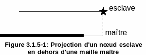
Figure 3.1.5-1: Projecting a slave node outside of a master mesh

One solution then consists in not pairing the node, which is tantamount to excluding it from contact:

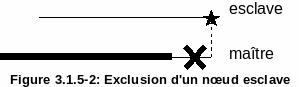
Figure 3.1.5-2: Excluding a slave node

However, this solution does not take into account borderline cases and may cause untimely interpenetrations if the mesh is not « optimal » (i.e. not fine enough, which is difficult to ensure in the context of large transformations). On the contrario, it is obviously not possible to fold down all the knots projecting outside the master surface.

An intermediate solution was therefore opted for by limiting the extension of the master surface liable to cause drawdown.

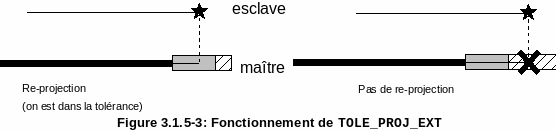
Figure 3.1.5-3: How TOLE_PROJ_EXT works

The size of the drawdown zone is fixed by the keyword “TOLE_PROJ_EXT” which takes as argument the value, in relation to the reference element, of the extension of the master mesh. By default, this value is set to 0.50. For example in 2D, this means that any slave node projecting more than 25% to the right or left of the length of the master mesh will not be pulled down (in the case of a segment, the reference element is of length 2, cf. [R3.01.01]). To completely forbid drawdown, simply fix negative TOLE_PROJ_EXT. This operator is valid in 2D and 3D (in the latter case, it is the extension of a surface contact mesh).

Note:

It is dangerous to completely deactivate the drawdown. Apart from the edges of the contact surfaces, there are in fact situations where points do not project into any master mesh (this is the case for any convex master surface). If all contact nodes were excluded, an alarm is issued. It is then necessary to verify that this situation is in fact the one expected by the user.

3.1.6. Choice of normals#

3.1.6.1. Normal type (NORMALE)#

66/ NORMALE = /” MAIT “[DEFAUT]

/”MAIT_ESCL” /”ESCL”

It is possible to choose the type of normal used to write the non-interpenetration conditions:

the normal outside of the master mesh (NORMALE =” MAIT “, by default);
the internal normal to the slave mesh (NORMALE =” ESCL “);
an average between the normal master and slave (NORMALE =” MAIT_ESCL “).

3.1.6.2. Determining master or slave normals (VECT_MAIT/VECT_ESCL)#

66/ VECT_MAIT = /” AUTO “[DEFAUT]

/”FIXE” /”VECT_Y” ♦ MAIT_FIXE = (Yx,Yy,Yz) [R] ♦ MAIT_VECT_Y = (Yx,Yy,Yz) [R]

66/ VECT_ESCL = /” AUTO “[DEFAUT]

/”FIXE” /”VECT_Y” ♦ ESCL_FIXE = (Yx,Yy,Yz) [R] ♦ ESCL_VECT_Y = (Yx,Yy,Yz) [R]

The determination of the normal (on the slave mesh or on the master mesh) can be done in several ways:

automatically, the normal is then calculated by using the element’s shape functions, this is the “AUTO” option;
fixed and given directly by the user, this is the “FIXE” option. We then enter normal with the keyword MAIT_FIXE or ESCL_FIXE;
variable and given indirectly by the tangent, this is option VECT_Y. The user then gives the direction of the**second tangent vector** with the keyword MAIT_VECT_You ESCL_VECT_Y. The code then reconstructs the normal from the vector product of the first tangent of the mesh and the vector provided by the user.

A fixed direction (option VECT_ *=” FIXE “) is necessary if we need to evaluate the normal on a POI1 mesh.

A variable direction given by the second tangent (VECT_MAIT =” VECT_Y “) is particularly used in the case of beams that only deform in one plane. In this case, using the VECT_Ypermet type option to continuously update the normal while the beam deforms:

\(\vec{N}=\vec{T}\wedge \mathit{VECT}\text{\_}Y\)

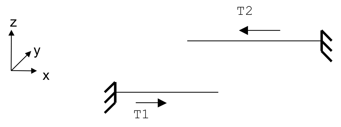
Figure 3.1.6.2-1: Determining the normal by VECT_Y

In the example above, T1= (1,0,0) and T2= (-1,0,0), with VECT_Y =( 0,1,0), we get the desired normal for each beam: N1 =( 0,0.1) and N2 =( 0,0, -1) and N2 =( 0,0, -1).

The orientation of each beam (i.e. the vectors T1 and T2) is given using the ORIE_LIGNE keyword from the MODI_MAILLAGE operator [U4.23.04].

3.1.6.3. Smoothing normals (LISSAGE)#

* LISSAGE = /” NON “, [DEFAUT]

/”OUI”,

The LISSAGE operand makes it possible to smooth the normals to the contact surfaces involved in the calculation of the contact matrix. Note \(Q\) any node of the contact surfaces (master or slave), \(P\) a node of the slave surface and \(M\) the master node obtained by projecting the node \(P\).

Smoothing is done in two steps:

the first step in smoothing consists in averaging at node \(Q\) the normals to the meshes that contain \(Q\);
the second step consists in interpolating the normal in \(P\) or \(M\) from the normals in \(Q\) and the shape functions associated with the mesh containing \(P\) or \(M\).

The smoothing takes into account the normal options decided by the keywords VECT_MAIT and VECT_ESCL. Attention, this parameter is global and not zoned.

3.1.7. Game modification#

The game is always calculated as being the minimum distance between the slave node and the projection on the nearest master mesh, modulo the options for choosing this normal (cf. 3.1.6). However, it is possible to define « hard » game values, for example, to simulate the presence of a hole or a bump not represented by the mesh, or to take into account the geometric characteristics of structural elements that use the concept of neutral fiber or average surface.

3.1.7.1. Operands DIST_MAIT/DIST_ESCL#

mary DIST_MAIT = dist_[ function]

◊ DIST_ESCL = dist_escl [fonction]

These operands make it possible to take into account a fictional non-mesh game or the thickness of the shells for example (by default the contact relationships are written between the parts meshed, i.e. between the two middle sheets).

This game is taken into account on master (DIST_MAIT) or slave (DIST_ESCL) surfaces. The distance is counted positively in the direction of the outgoing normal to the structure (cf. [R5.03.50]). A negative value therefore makes it possible to virtually « dig » a surface (master and slave). On the other hand, a positive value makes it possible to « increase » an area.

The quantities entered are necessarily functions of the variables of space or time (\(X,Y,Z,\mathit{INST}\)). If the user wants a fixed value, he must define a constant function (see DEFI_CONSTANTE [U4.31.01]).

3.1.7.2. Operands DIST_POUTRE/DIST_COQUE/CARA_ELEM#

66/ DIST_POUTRE = /” NON “[DEFAUT]

/”OUI”

66/ DIST_COQUE = /” NON “[DEFAUT]

/”OUI”

♦ CARA_ELEM = character [cara_elem]

Similar to the two previous keywords, the keywords DIST_POUTRE/DIST_COQUE make it possible to introduce a fictional game that is based on the description of the structural elements in the concept produced by AFFE_CARA_ELEM that the user must have filled in:

for beam elements (modeling POU_*), the DIST_POUTRE keyword states that the code must take into account an additional gap corresponding to the radius of the circular section of the beam.
for plate or shell elements (modeling DKTou COQUE_3Dpar example), the keyword DIST_COQUE states that the code must take into account an additional gap corresponding to the half-thickness around the middle sheet of a shell.

Attention, when using these keywords, the fictional game is only added to the slave surface. If we model a contact between two structural elements, we must therefore also use DIST_MAIT.

3.2. Formulation-specific pairing control CONTINUE#

3.2.1. Operands SANS_GROUP_NO_FR#

* SANS_GROUP_NO_FR = l_sgrno [l_gr_node]

◊ DIRE_EXCL_FROT = (Yx, Yy, Yz) [R]

These keywords allow the user to exclude slave nodes carrying boundary conditions potentially in conflict with the imposition of grip and slip conditions from the friction treatment. However, the excluded nodes continue to check the contact conditions.

In 2D, no other keywords are needed: knots are excluded from friction.

In 3D, if the user has entered a 3-component vector under the keyword DIRE_EXCL_FROT then the direction indicated by the projection of this vector on the tangential plane at the contact points is excluded. Adhesion or sliding will therefore only occur in the perpendicular direction (in the tangential plane).

If the user does not enter the keyword DIRE_EXCL_FROT in 3D, then this amounts to excluding the 2 orthogonal directions of the friction and therefore to no longer resolving the friction on the eliminated nodes.

Note:

Excluding nodes is only possible with the integration scheme by default (cf. § 3.5.2.4 )

3.3. Formulation-specific control LAC#

♦ ZONE = _F (options)

The keywords in this paragraph are valid for the LAC method.

3.3.1. Operands GROUP_MA_MAIT/GROUP_MA_ESCL#

♦/GROUP_MA_MAIT = l_grma_ait [l_gr_mesh]

♦/GROUP_MA_ESCL = l_grma_escl [l_gr_mesh]

For the formulation LAC the user provides the list of potential contact meshes of the master surface (GROUP_MA_MAIT) and the slave surface (GROUP_MA_ESCL). The slave surface must have been prepared beforehand (cut into patches) by the CREA_MAILLAGE/DECOUPE_LAC command.

Care:

It is important to check that the connectivity of these meshes is such that **the normal to the structure is outgoing (to do this, use* MODI_MAILLAGE keyword ORIE_PEAU_2D, , ORIE_PEAU_3D, , , , ORIE_NORM_COQUE [U4.23.04]).
The intersection between slave and master surfaces in the same zone must be disjoint or the common nodes must be excluded (cf. 3.1.3 ) .
The slave surfaces must be separated two by two

3.3.2. Operands APPARIEMENT/TYPE_APPA#

* APPARIEMENT = /” MORTAR “[DEFAUT]

* TYPE_APPA = /” ROBUSTE “[DEFAUT]

/”RAPIDE”

mary RESI_APPA = /1.0E-8 [DEFAUT]

/resi_appa: [R]

Method LAC necessarily uses a « mortar » pairing, i.e. segment/segment (in 2D) or face/face (in 3D). This pairing is much more expensive than a node/segment pairing used for other contact methods. We therefore have the choice between two possibilities:

Use an algorithm that is fast but may cause false pairings (it is easy to control this problem visually). We then choose TYPE_APPA = “RAPIDE”;
Use a robust but much slower algorithm. We then choose TYPE_APPA = “ROBUSTE;

It is recommended to use « fast » matching only for simple cases (related surfaces).

Parameter RESI_APPA allows you to adjust the degree of accuracy of the pairing. It is not recommended to touch it; its use requires great care and should be reserved for experts.

3.3.3. Operand TYPE_JACOBIEN#

66/ TYPE_JACOBIEN = /” INITIAL “[DEFAUT]

/” ACTUALISE “

This operand is used when the kinematics of the problem are of the « large transformations » type. For example, if you do a simulation with the « GDEF_LOG » model, you must use TYPE_JACOBIEN =” ACTUALISE “, otherwise the results (in particular contact pressures) will be slightly wrong.

3.3.4. Operand CONTACT_INIT#

* CONTACT_INIT = /” INTERPENETRE “[DEFAUT]

/”OUI” /”NON”

* SEUIL_INIT =/0. [DEFAUT]

/seuil_init: [R]

The CONTACT_INIT operand allows you to set the contact status to the initial state.

By default, only zero-clearance or well-interpenetrated links are activated by the algorithm (CONTACT_INIT =” INTERPENETRE “). However, it is possible to force the algorithm to activate all links without exception (CONTACT_INIT =” OUI “). The value CONTACT_INIT =” INTERPENETRE “is mandatory in case of resuming the calculation with an initial state. It is also possible to deactivate any initial contact by CONTACT_INIT =” NON “.

The LAC method uses a specific output data structure, CONT_ELEM, defined by element (see § 3.7).

3.4. Choice and control of the global resolution algorithm#

3.4.1. Geometric nonlinearity check#

Whatever the formulation used, it is necessary to deal with the geometric nonlinearity of the touch-friction problem. It is possible either to ignore it (REAC_GEOM =” SANS “), or to solve it in an approximate way (REAC_GEOM =” CONTROLE”) or exactly (REAC_GEOM =” AUTOMATIQUE “).

To solve this nonlinearity, a « fixed point » algorithm is generally used (ALGO_RESO_GEOM =” POINT_FIXE “). The formulation CONTINUE is also capable of dealing with geometric nonlinearity within the Newton algorithm itself (ALGO_RESO_GEOM =” NEWTON “, see § 3.4.4.5).

When geometric nonlinearity is resolved by a « fixed point » loop, a number of adjustments are possible:

◊ REAC_GEOM = /' AUTOMATIQUE ', [DEFAUT]

/” CONTROLE “, /” SANS “

* ITER_GEOM_MAXI = /10, [DEFAUT]

/iter_geom_maxi, [I]

◊ RESI_GEOM = /0.01, [DEFAUT]

/0.0001, [DEFAUT] (XFEM) /resi_geom, [R]

◊ NB_ITER_GEOM = /2, [DEFAUT]

/nb_iter_geom, [I]

The operand REAC_GEOM indicates on which geometric configuration the contact problem is treated:

REAC_GEOM =” AUTOMATIQUE “: the geometry is automatically updated, i.e. the number of « geometric update-iterations » cycles until convergence is not fixed in advance but obeys a criterion of geometric convergence. This is the default option, recommended to resolve pairing nonlinearity correctly. It ensures that the contact conditions have been imposed on a configuration (initial) that differs by less than resi_geom from the configuration found (1% by default for formulations DISCRETE or CONTINUE).
REAC_GEOM =” SANS “: we are working on the initial geometry. This option is only valid if there are small disturbances or when the normal to the contact surfaces does not change during the calculation.
REAC_GEOM =” CONTROLE “: when the automatic criterion cannot be satisfied, the user must check the geometric update himself and for this he must enter the parameter NB_ITER_GEOM. This is the number of geometric refresh cycles that will be carried out per load step. Let’s place ourselves at a given load step:
- The value 1 indicates that at Newton convergence, we update the geometry and move on to the next load step.
- The value 2 indicates that at Newton convergence, the geometry is updated and repeated until convergence before moving on to the next load step.
- The value \(n>2\) indicates that \(n\) « geometric refresh-convergence » cycles are done before moving on to the next load step.

If you selected REAC_GEOM =” AUTOMATIQUE “, the parameter ITER_GEOM_MAXI is the maximum allowed number of geometric refresh cycles. If the criterion relating to RESI_GEOM is not satisfied after iter_geom_maxi cycles, then we stop in error or we cut the time step if the user has requested it. The [U2.04.04] documentation provides numerous tips for overcoming these convergence problems (in particular, enabling smoothing).

Remarks:

If the user chooses a controlled refresh with \(n>1\) and Code_Aster detects the need for a geometric refresh, it will sound an alarm. It is up to the user to decide whether the error committed (necessarily greater than 1%) is acceptable or not. There is in fact a risk of pairing error (a mesh has been matched on a configuration that has moved) and therefore of interpenetration.
In the case where we solve on the initial geometry or with a single geometric update cycle, there is no warning because we cannot calculate an error. The user must therefore check the validity of his choice during post-processing.
The value of the geometric convergence criterion is shown in the Newton iteration table (column CONTACT CRITERE VALEUR ) .

3.4.2. Friction#

◊ FROTTEMENT = /' SANS ', [DEFAUT]

/” COULOMB “,

To assign Coulomb friction to contact areas, use the keyword FROTTEMENT =” COULOMB “. This keyword is global (valid for all zones), but it is possible to assign friction zone by zone by playing on the value of the Coulomb coefficient (you set this coefficient to 0 when you do not want friction).

3.4.3. Formulation DISCRETE#

3.4.3.1. Choice of algorithms#

♦ ALGO_CONT = /” CONTRAINTE “[DEFAUT]

/”GCP” /”PENALISATION”

♦ ALGO_FROT = /” PENALISATION “[DEFAUT]

To select the type of algorithm in the formulation DISCRETE, the keywords ALGO_CONT and ALGO_FROT are used. ALGO_FROT can only be changed if FROTTEMENT =” COULOMB “. Not all combinations are possible:

	ALGO_FROT =” PENALISATION “
ALGO_CONT =” CONTRAINTE “	**Impossible
ALGO_CONT =” GCP “	**Impossible
ALGO_CONT =” PENALISATION “	OK

The various resolution methods are:

“CONTRAINTE “:default algorithm that treats the problem of exact one-sided contact with the active constraints method (see [R5.03.50]).**No friction possible **.
“GCP”: it is an iterative method similar to the “CONTRAINTE” method but which is particularly suitable for cases where the number of contact links is very high.**No friction possible **.
“PENALISATION “:the penalized method makes it possible to deal with contact problems in an approximate manner with or without friction, in 2D or 3D.

Although the different algorithms are given by zone, it is not possible to mix several methods in the same DEFI_CONTACT.

3.4.3.2. Dualized methods (CONTRAINTE)#

Method CONTRAINTE makes it possible to solve contact problems without friction in an exact manner (no interpenetration is tolerated). It is particularly fast and robust; its convergence has been proven. Since the resolution of the system of inequalities resulting from contact is based on the explicit construction of a Schur complement, its use is limited to a few hundred contact links. Beyond that, memory and computation costs are becoming too important.

66/ NB_RESOL = /10, [DEFAUT]

/nb_resol: [I]

NB_RESOLest the number of simultaneous resolutions for building the Schur complement. Performing several simultaneous resolutions makes it possible to manipulate matrices by blocks. Increasing nb_resol therefore speeds up the construction of the Schur complement but wastes memory space. nb_resol=10 is a good compromise. This setting is for experts only.

* STOP_SINGULIER = /” OUI “, [DEFAUT]

/”NON”

STOP_SINGULIER allows you to deactivate the fatal error that occurs if the Schur complement is singular following a significant loss of decimals in factorization (8 decimals by default). To do this, we fill in STOP_SINGULIER =” NON “. This setting is for experts only.

* ITER_CONT_MULT = /4, [DEFAUT]

/iter_cont_mult, [I]

You can control the status loop by giving a multiplier coefficient, ITER_CONT_MULT: the maximum number of iterations on the contact status will be equal to the product iter_cont_multby the number of slave nodes.

If the calculation stops because the maximum number of contact iterations is exceeded, we can then try to refine the mesh, subdivide the time step or as a last resort increase the value of ITER_CONT_MULT.

Note: for method CONTRAINTE, the convergence being proved, this coefficient is fixed hard to 2.

3.4.3.3. Method GLISSIERE#

66/ GLISSIERE = /” NON “[DEFAUT]

/”OUI”

66/ ALARME_JEU = /0 [DEFAUT]

/alarme_jeu: [R]

This option is only available for the “CONTRAINTE” method. It makes it possible to activate the bilateral contact mode, also called « slide », in which two surfaces in contact remain « stuck » (i.e. with zero play) regardless of the evolution of the load. It allows large relative changes.

Bilateral contact is only activated once the surfaces are actually in contact (one does not stick a priori two separate surfaces if the loading does not involve it).

The operand “ALARME_JEU” makes it possible to trigger an alarm as soon as the algorithm detects that, without the slide method, there would be detachment of the two surfaces. Its value is set by default to 0, which alerts the user as soon as the surfaces should have come off without the option activated.

3.4.3.4. Method GCP#

This method makes it possible to solve contact problems without friction. It solves contact conditions with adjustable precision (possibly very high) using Lagrange multipliers. It is in every way similar to the “CONTRAINTE” method except that it is completely iterative in nature and therefore very low in memory. In other words, the additional storage cost associated with taking contact into account is low. This specificity has the effect of making it particularly suitable for cases involving a large number of contact links.

66/ RESI_ABSO = /resi_abso [R]

66/ ITER_GCP_MAXI = /0 [DEFAUT]

/iter_gcp_maxi

◊ RECH_LINEAIRE = /” ADMISSIBLE “[DEFAUT] /” NON_ADMISSIBLE “ ◊ PRE_COND = /” SANS “, [DEFAUT] /” DIRICHLET “

66/ ITER_PRE_MAXI = /0 [DEFAUT]

/iter_pre_maxi: * COEF_RESI = /-1. [DEFAUT]

/coef_resi: [R]

The RESI_ABSO keyword allows you to adjust the precision of the resolution of contact inequalities (it is a criterion for stopping the value of the games for the iterative algorithm). RESI_ABSO (which should be understood by « absolute residue ») represents the maximum level of interpenetration tolerated for bodies in contact. From a practical point of view, we will start by choosing a value of the order of \({10}^{-3}\) times the size of the elements in the vicinity of the contact surfaces and then we will reduce this value until the results stabilize.

The maximum number of allowed iterations of the projected conjugate gradient algorithm can be set with the ITER_GCP_MAXI keyword. By default, this number of iterations depends on the size of the problem.

Like any iterative resolution method, the 'GCP' method can be accelerated by using a preconditioner. Only one is available today: a Dirichlet pre-conditioner (PRE_COND =' DIRICHLET '). In some cases, its use can significantly speed up and reduce the resolution time. By default no preconditioner is activated (PRE_COND =' SANS ').

The pre-conditioning phase is carried out by the resolution (also iterative) of an auxiliary problem. The keyword COEF_RESI makes it possible to trigger this preconditioner only when the residue has sufficiently decreased: more precisely when the initial residue of the algorithm (i.e. the initial interpenetration) has been multiplied by coef_resi (coef_resi is therefore smaller than 1).

ITER_PRE_MAXIpermet to set the maximum number of iterations of the preconditioner.

The 'GCP' resolution method requires a phase called linear search. Two variants are available: eligible or ineligible. They are chosen with the keyword RECH_LINEAIRE (cf. [R5.03.50]).

3.4.3.5. Method PENALISATION#

This method is a method for resolving touch/friction by regularization. It is inaccurate in the sense that there is always interpenetration when contact is established. If a discrete formulation with penalization is used, it is therefore appropriate to enter the penalty coefficient (s) (see § 3.5.1.1).

3.4.4. Formulation CONTINUE#

3.4.4.1. Choice of algorithms#

***** ALGO_RESO_CONT = /' NEWTON '[DEFAUT]

/”POINT_FIXE”

* ALGO_RESO_FROT = /” NEWTON “[DEFAUT]

/”POINT_FIXE”

* ALGO_RESO_GEOM = /” POINT_FIXE “[DEFAUT]

/”NEWTON”

3.4.1: The continuous formulation has two types of algorithms to solve the non-linearities of touch-friction: fixed point algorithm or generalized Newton algorithm. In addition to geometric nonlinearity (see §), this choice can also be made for contact and friction nonlinearity via the keywords ALGO_RESO_CONT, ALGO_RESO_FROT and ALGO_RESO_GEOM (not all choices are possible):

ALGO_RESO_CONT	ALGO_RESO_FROT	ALGO_RESO_GEOM
POINT_FIXE	POINT_FIXE	POINT_FIXE	OK
NEWTON	POINT_FIXE	POINT_FIXE	OK
POINT_FIXE	NEWTON	POINT_FIXE	OK
NEWTON	NEWTON	POINT_FIXE	OK (by default)
POINT_FIXE	POINT_FIXE	NEWTON	**Impossible
NEWTON	POINT_FIXE	NEWTON	OK
POINT_FIXE	NEWTON	NEWTON	**Impossible
NEWTON	NEWTON	NEWTON	OK

When we choose the generalized Newton method for friction, the tangent matrix produced becomes non-symmetric. The generalized Newton method is much faster and less sensitive to the value of the coefficient of friction than the fixed point method. In some cases, it may prove to be less robust in the treatment of geometric nonlinearity, which is why it is not activated by default in this case. In the case of solving a generalized Newton touch-friction problem, it is often necessary to increase the number of iterations of Newton (set by default to 10).

Regardless of the resolution method used (fixed point or Newton) the results obtained are identical.

Note:

The option MATR_DISTRIBUEE =” OUI “of the keyword factor SOLVEUR non-linear operators is forbidden with contact in continuous formulation.

3.4.4.2. Contact nonlinearity#

***** ITER_CONT_TYPE = /' MAXI ', [DEFAUT]

/”MULT”

* ITER_CONT_MULT = /4, [DEFAUT]

/iter_cont_mult, [I]

◊ ITER_CONT_MAXI = /30, [DEFAUT]

/iter_cont_maxi, [I]

With the default settings (ALGO_RESO_CONT =' NEWTON '), there are no parameters to provide for the resolution of contact nonlinearity.

When you choose ALGO_RESO_CONT =' POINT_FIXE ', you can control the contact status loop in two ways:

Giving the maximum**absolute** number of contact iterations, ITER_CONT_TYPE =” MAXI “then ITER_CONT_MAXI;
By giving the maximum**relative** number of contact iterations by a multiplier coefficient, ITER_CONT_TYPE =” MULT “then ITER_CONT_MULT; in this case, the number of iterations on the contact status will be equal to the product iter_cont_multby the number of slave nodes.

In the fixed point method, the statuses are changed in blocks and the maximum number of iterations is therefore more logically entered in absolute value. If the maximum number of contact iterations is reached, we can then try to refine the mesh, subdivide the time step, or as a last resort increase the value of ITER_CONT_MAXI/ITER_CONT_MULT.

3.4.4.3. Stabilization of contact statuses with elastic matrix#

* CONT_STAT_ELAS = /0, [DEFAUT]

/cont_stat_elas, [I]

The keyword allows you to activate the use of the elastic matrix (even if MATRICE = « TANGENTE » under NEWTONdans STAT_NON_LINE) during iterations of the correction phase of Newton’s algorithm until the contact statuses are stabilized during cont_stat_elas iterations. By default, this feature is not active, cont_stat_elas=0. Using this feature can be useful when modeling contact with non-linear behaviors and when there are failures to integrate the law of behavior when stabilizing statuses.

3.4.4.4. Non-linearity of friction threshold#

* ITER_FROT_MAXI = /10, [DEFAUT]

/iter_frot_maxi, [I]

◊ RESI_FROT = /0.0001, [DEFAUT]

/resi_frot, [R]

By default the Coulomb problem is solved by a generalized Newton algorithm (ALGO_RESO_FROT =” NEWTON “), the only keyword that can be entered is therefore RESI_FROT to define the threshold stationarity criterion (during of RESI_GEOM, cf. 3.4.1). An additional column in the convergence table makes it possible to track the value of the criterion (column CONTACT NEWTON GENE CRIT). FROT .).

When we choose ALGO_RESO_FROT =” POINT_FIXE “, the Coulomb problem is solved by a succession of fixed points on the Tresca threshold. To control this loop, the mechanism is the same as on the geometric update loop (cf. 3.4.1, ITER_FROT_MAXI plays the role of ITER_GEOM_MAXI and RESI_FROT plays the role of RESI_GEOM).

When you choose ADAPTATION = ADAPT_COEF, you activate the possibility of controlling the coefficient of increase in friction (COEF_FROT) by an automatic cycle processing method (see [R5.03.52]). This option should be activated in case of convergence difficulties if the generalized Newton method is used, in the case where a large number of cycles occur. The number of cycles during an iteration is shown in column CONTACT INFOS CYCLAGES in the convergence table.

3.4.4.5. Geometric nonlinearity#

◊ RESI_GEOM = /0.000001, [DEFAUT]

/resi_geom, [R]

The parameters of the fixed point loop on the geometry (setting by default) are given in § 3.4.1.

When we choose ALGO_RESO_GEOM =” NEWTON “, we switch to the generalized Newton algorithm. Geometric non-linearity is then taken into account at each Newton’s iteration: the pairing is done again and the local base is recalculated (normal and tangents). In this mode, an additional column appears in the convergence table, it corresponds to the evaluation of the geometric criterion (column CONTACT NEWTON GENE CRIT). GEOM .).

It is possible to change the target value of this criterion, just like in the POINT_FIXE mode, using the RESI_GEOM parameter. However, its definition in generalized Newton implies that it is generally verified before Newton’s equilibrium criterion. If you really want to control it, you have to switch to POINT_FIXE mode.

3.4.5. Formulation XFEM#

3.4.5.1. Fixed point loop for contact statuses#

***** ITER_CONT_TYPE = /' MAXI ', [DEFAUT]

/”MULT”

66/ ITER_CONT_MULT = /4, [DEFAUT]

/iter_cont_mult, [I]

◊ ITER_CONT_MAXI = /30, [DEFAUT]

/iter_cont_maxi, [I]

You can control the contact status loop in two ways:

Giving the maximum**absolute** number of contact iterations, ITER_CONT_TYPE =” MAXI “then ITER_CONT_MAXI;
By giving the maximum**relative** number of contact iterations by a multiplier coefficient, ITER_CONT_TYPE =” MULT “then ITER_CONT_MULT; in this case, the number of iterations on the contact status will be equal to the product iter_cont_multby the number of slave nodes.

For the formulation XFEM, the statuses are changed in blocks and the maximum number of iterations is therefore more logically entered in absolute value. In all cases, changing these parameters is reserved for experts because it can lead to false results if friction is activated.

If we exceed the maximum number of contact iterations, we can then try to refine the mesh, subdivide the time step, or as a last resort increase the value of ITER_CONT_MAXI/ITER_CONT_MULT.

3.4.5.2. Fixed point loop for friction#

***** ITER_FROT_MAXI = /10, [DEFAUT]

/iter_frot_maxi, [I]

◊ RESI_FROT = /0.0001, [DEFAUT]

/resi_frot, [R]

For the formulation XFEM (in small slips), the Coulomb problem is solved by a succession of fixed points on the Tresca threshold. To control this loop, the mechanism is the same as on the geometric update loop.

For X- FEM in big swings (REAC_GEOM! =” SANS “), there is no loop on the Tresca thresholds (generalized Newton algorithm). Parameter ITER_FROT_MAXI then has no effect.

3.4.5.3. Managing redundant edges#

* ELIM_ARETE = /” DUAL “, [DEFAUT]

/”ELIM”

In the theoretical documentation of XFEM taking into account touch/friction [R5.03.04], we explain the importance of eliminating certain edges cut by the level-set to respect the inf-sup stability condition (or condition LBB). This algorithm consists in establishing linear relationships (equalities) between certain degrees of freedom. By activating ELIM_ARETE =” ELIM “, these relationships are written in explicit form and redundant degrees of freedom are eliminated from the unknowns, which is more efficient (smaller model, less risk of conditioning problems). In some situations, this method may fail. In this case, all you have to do is go back to mode ELIM_ARETE =” DUAL “.

3.4.6. Method without resolution#

* STOP_INTERP = /” NON “, [DEFAUT]

/”OUI”

In the case of the mode without resolution (see § 3.5.4) the code emits an alarm as soon as it detects an interpenetration. The STOP_INTERP parameter allows you to stop the calculation instead of alarming the user.

3.5. Local resolution control settings (zone by zone)#

3.5.1. Local parameters (zone by zone) from formulation DISCRETE#

♦ ZONE =_F (local settings)

The keywords in this paragraph are valid for the formulation DISCRETE. The settings are set by zone.

3.5.1.1. Method “PENALISATION”#

♦ E_n = e_n [R]

♦ E_T = e_t [R]

e_n is the penalty coefficient on interpenetration for the penalized method. It is homogeneous in a ratio of forces per length: it is the stiffness of springs placed between the contact surfaces to prevent interpenetration. A value of the order of the greatest Young’s modulus of the solids in contact multiplied by a characteristic length is initially recommended. The value of the coefficient will be increased until stable results are obtained.

In addition, it is possible to control the interpenetration distances and therefore to refine one’s choice of coefficient, which is not the case in the presence of friction, since one does not know a priory which are the slippery and non-sliding zones, whereas in the event of contact it is possible to verify that the interpenetration distances are small compared to the characteristic dimensions of the contact zones.

In formulation DISCRETE, there is a mechanism for automatically adapting the penalty coefficient E_N (cf. DEFI_LIST_INST [U4.34.03]).

e_t is the slippage penalty coefficient for the penalized method. It is homogeneous in a ratio of forces by length. It is only needed when the contact is active. The value of this coefficient must be increased until stable results are obtained, i.e. results that depend as little as possible on it.

3.5.1.2. Specific parameters for friction#

♦ COULOMB = coulomb [R]

◊ COEF_MATR_FROT = coef_matr_frot [R]

Parameter COULOMB allows you to adjust the coefficient of friction.

In the case of a penalized formulation, the parameter COEF_MATR_FROT, between 0 and 1, makes it possible to moderate the destabilizing effect of the negative part of the sliding matrix (which is added to the tangent stiffness, cf. [R5.03.50]). The greater this coefficient, the better the convergence when one is close to equilibrium and the more difficult it is to resolve far from equilibrium. A value of 0.5 is therefore a good compromise. The default value set to 0 ensures better robustness for a longer calculation time.

3.5.2. Local parameters (zone by zone) from formulation CONTINUE#

♦ ZONE =_F (local settings)

The keywords in this paragraph are valid for the formulation CONTINUE. The settings are set by zone.

3.5.2.1. Operands CONTACT_INIT/SEUIL_INIT#

* CONTACT_INIT = /” INTERPENETRE “[DEFAUT]

/”OUI” /”NON”

* SEUIL_INIT =/0. [DEFAUT]

/seuil_init: [R]

The operands CONTACT_INIT and SEUIL_INIT make it possible to set the contact status to the initial state and the initial sliding threshold respectively.

With regard to friction, the user can specify, if he wishes, the value of the initial threshold (if he wants an initial adherent contact for example). The sliding threshold has the dimension of a surface force density. At a point on the contact surface, there will be slippage if the contact pressure \(\mathrm{\lambda }\) and the coefficient of friction \(\mathrm{\mu }\) satisfy: \(\mathrm{\lambda }⩾\mathrm{\mu }\times \mathit{SEUIL}\text{\_}\mathit{INIT}\). The value he has chosen will apply to all points in the contact area concerned. If no value is specified then the default behavior of SEUIL_INIT is as follows:

if it is a repeat calculation or a calculation with initial state, then the initial threshold field of each contact point is automatically reconstructed using the values of the component LAGS_C of the field DEPLprécisé in field in STAT_NON_LINE/ETAT_INIT,
otherwise, the initial threshold is set to zero and all points are potentially slippery.

3.5.2.2. Coefficient for formulation CONTINUE#

* ALGO_CONT = /” STANDARD “[DEFAUT]

/”PENALISATION” {Si ALGO_CONT== “STANDARD” ♦ COEF_CONT = /100. [DEFAUT] /coef_cont [R] }}}} {Si ALGO_CONT== “PENALISATION’Et ADAPTATION=”NON” ou “CYCLAGE” ♦ COEF_PENA_CONT = coef_pena_cont [R] }}}} {Si ALGO_CONT== “PENALISATION’Et ADAPTATION=”PENE_MAXI” ou “TOUT” ◊ PENE_MAXI= coef_pena_cont [R] }}}}

* ALGO_FROT = /” STANDARD “[DEFAUT]

/”PENALISATION” {Si ALGO_FROT== “STANDARD” ♦ COEF_FROT = /100. [DEFAUT] /coef_frot [R] }}}} {Si ALGO_FROT== “PENALISATION” ♦ COEF_PENA_ FROT= coef_pena_frot [R]

}

The continuous formulation is an augmented Lagrangian formulation. There is a penalized version.

If we choose ALGO_CONT =” STANDARD “and ALGO_FROT =” STANDARD” and =” “, the continuous formulation is then equivalent to a conventional augmented Lagrangian formulation whose increase coefficients are given, respectively, by COEF_CONT and COEF_FROT.

If we choose ALGO_CONT =” PENALISATION “and ALGO_FROT =” PENALISATION”, the wording is then a penalized Lagrangian. We can then modify the penalty coefficients COEF_PENA_CONT and COEF_PENA_FROT but only when we choose ADAPTATION =” NON “or ADAPTATION =” CYCLAGE”.

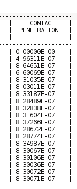
In the case where we want to use the automatic penalty mode ADAPTATION =” TOUT “or ADAPTATION =” ADAPT_COEF”, we no longer worry about choosing COEF_PENA_CONT but only with PENE_MAXI. If PENE_MAXI is not specified, then by default PENE_MAXI is equal to \(1.0\phantom{\rule{2em}{0ex}}{10}^{-2}\) times the smallest edge value in the contact area. The maximum penetration value over all contact areas is entered in the « CONTACT PENETRATION » column. This indicates the quality of treatment due to the penalized method.

You can also use mixed modes ALGO_CONT =” STANDARD “and ALGO_FROT =” PENALISATION” and vice versa.

The penalized method is described in the case of the discrete method in § 3.4.3.5 and § 3.5.1.1, COEF_PENA_CONT corresponds to E_N and COEF_PENA_FROT to E_T.

3.5.2.3. Operand ADAPTATION#

* ADAPTATION = /” CYCLAGE “[DEFAUT]

/”ADAPT_COEF” /”TOUT” /”NON”

The operand “ADAPTATION” makes it possible to select a method for dealing with cases of convergence that is difficult for the contact:

“NON”: there is no treatment;
“ADAPT_COEF”: we automate the calculation of COEF_PENA_CONT and/or COEF_PENA_FROT;
“CYCLAGE”: frequent changes in contact statuses can make convergence difficult. To avoid these untimely changes in status (« we talk about « cycling »), we modify the calculation of the contact and friction matrices. The contact matrix becomes a convex combination between the state matrices (pressure, play, status) of the contact point cycling at the previous iteration and at the current iteration. This mode is available for ALGO_CONT =” STANDARD “/” PENALISATION “/” LAC “. In addition, in this mode, an automatic and definitive switch between the mode ALGO_CONT =” STANDARD “and the mode ALGO_CONT =” PENALISATION” may occur if the contact statuses do not converge well. In this case, there will be automatic control of maximum penetration (keyword PENE_MAXI);
“TOUT”: we combine the “CYCLAGE” mode with the “ADAPT_COEF” mode;

3.5.2.4. Operand INTEGRATION#

* INTEGRATION = /” AUTO “[DEFAUT]

/”GAUSS” /”SIMPSON” /”NCOTES”

{If INTEGRATION == “GAUSS” ◊ ORDRE_INT = /3 [DEFAUT] /1 ≤int_order ≤6 [I] }}}} {If INTEGRATION == “SIMPSON” ◊ ORDRE_INT =/1 [DEFAUT] /1 ≤int_order ≤4 [I] }}}}

{If INTEGRATION == “NCOTES”

◊ ORDRE_INT = /3 [DEFAUT] /3≤ordre_int ≤8 [I]

The operand “INTEGRATION” makes it possible to select a numerical integration method for the terms of contact and friction. Several methods are implemented:

“AUTO” to let the code choose the most suitable integration scheme (trapezoid or Simpson type);
“GAUSS” for a Gauss quadrature with the possibility of choosing the degree of the polynomials that the diagram allows you to integrate exactly;
“SIMPSON” for a Simpson diagram (\(1/3\)) with the possibility of choosing the number of subdivisions of the reference element;
“NCOTES” for a Newton-Cotes diagram with the possibility of choosing the degree of the interpolator polynomials.

The choice of the degree of the polynomials that we integrate exactly or the number of subdivisions for the Simpson diagram is made with the keyword ORDRE_INT.

Automatic integration (choice by default) is the most general and the most effective. The choice of an integration scheme is reserved for experts.

3.5.2.5. Operand GLISSIERE#

* GLISSIERE = /” NON “[DEFAUT]

/”OUI”

Contrary to the discrete formulation (see § 3.4.3.3), it is possible to activate this option zone by zone.

3.5.3. Local parameters (zone by zone) from formulation XFEM#

♦ ZONE = _F (local settings)

The keywords in this paragraph are valid for the formulation XFEM. The settings are set by zone.

3.5.3.1. Operand FISS_MAIT#

♦ FISS_MAIT = fiss_[ fiss_xfem]

For formulation XFEM, the user provides the crack that the lips will potentially come into contact with (FISS_MAIT). The expected concept comes from the operator DEFI_FISS_XFEM [U4.82.08].

3.5.3.2. Operands CONTACT_INIT/SEUIL_INIT#

* CONTACT_INIT = /” NON “[DEFAUT]

/”OUI”

* SEUIL_INIT =/0. [DEFAUT]

/seuil_init: [R]

Cf. 3.5.2.1.

3.5.3.3. Coefficient for formulation XFEM#

* ALGO_CONT = /” STANDARD “[DEFAUT]

/”PENALISATION” /”CZM” ◊ COEF_CONT = /100. [DEFAUT] /coef_cont [R] ◊ COEF_PENA_CONT = /100. [DEFAUT] /coef_pena_cont [R]

* ALGO_FROT = /” STANDARD “[DEFAUT]

/”PENALISATION” ◊ COEF_FROT = /100. [DEFAUT] /coef_frot [R] ◊ COEF_PENA_FROT = /100. [DEFAUT] /coef_pena_frot [R]

The formulation XFEMest is a continuous type of writing. The choice of coefficients is the same as in the case of the continuous formulation (§ 3.5.2.2).

The algorithm ALGO_CONT =” CZM “(Cohesive Zone Model) is particular. It is used when you want to model cohesive forces between two lips of a crack. Contact is then taken into account by a term of penalization in the cohesive law. The parameters relating to the law of touch-friction must then not be filled in. In fact, the parameter COEF_PENA_CONT is for example useless, the penalty coefficient being determined from the material parameters provided in the operator DEFI_MATERIAU [U4.43.01], under the keyword RUPT_FRAG. Since the tangential stress obeys the cohesive law and not a law of friction, no keywords concerning friction are used.

3.5.3.4. Operand INTEGRATION#

* INTEGRATION = /” NOEUD “[DEFAUT]

/”GAUSS” /”SIMPSON” /”NCOTES”

{If INTEGRATION == “GAUSS” ◊ ORDRE_INT = /6 [DEFAUT] /1 ≤int_order ≤6 [I] }}}} {If INTEGRATION == “SIMPSON” ◊ ORDRE_INT =/1 [DEFAUT] /1 ≤int_order ≤4 [I] }}}}

{If INTEGRATION == “NCOTES”

◊ ORDRE_INT = /3 [DEFAUT] /3≤ordre_int ≤8 [I]

}

This keyword has the same meaning as the phrase CONTINUE, cf. § 3.5.2.4. This is a parameter to be reserved for experts.

3.5.3.5. Operand GLISSIERE#

* GLISSIERE = /” NON “[DEFAUT]

/”OUI”

Contrary to the discrete formulation (see § 3.4.3.3), it is possible to activate this option zone by zone.

3.5.3.6. Operand ALGO_LAGR#

* ALGO_LAGR = /” AUTO “[DEFAUT]

/”VERSION1” /”VERSION2” /”VERSION3” /”NON”

This keyword determines the choice of the algorithm for eliminating friction Lagranges to satisfy condition LBB (see [R7.02.12]). This parameter is for use by experts. When the “AUTO” keyword is activated, for quadratic elements with REAC_GEOM == “SANS”, we switch to ALGO_LAGR == “VERSION3”. In all other cases, we activate ALGO_LAGR ==” VERSION2 “.

3.5.3.7. Operand RELATION#

◊ RELATION = /” CZM_EXP_REG “[DEFAUT]

/”CZM_LIN_REG” /”CZM_TAC_MIX” /”CZM_OUV_MIX” /”CZM_LIN_MIX”

The RELATIONpermet keyword to activate the consideration of cohesion forces when opening an X- FEM interface. It is used exclusively with the option ALGO_CONT = “CZM”. Cohesion is modelled by the cohesive law of the same name, already existing in classical finite element method (see the instructions for use [U2.05.07] for a summary, the documentation [R7.02.11] for the definition of these laws and the documentation [R5.03.54] for their extension to X- FEM). At present, the only law that can be used for propagation studies over an unknown path is CZM_LIN_MIX, a mixed law (perfect initial adherence) used with linear elements.

The necessary data for the material field is provided in the operator DEFI_MATERIAU [U4.43.01], under the keyword RUPT_FRAG.

3.5.4. Method without resolution#

* RESOLUTION = /” OUI “, [DEFAUT]

/” NON “

◊ TOLE_INTERP =/0., [DEFAUT]

/tole_interp [R]

When RESOLUTION =” NON “, the interpenetration of two surfaces is checked without imposing contact conditions (if there is interpenetration, it will not be corrected).

The code sounds an alarm as soon as an interpenetration is detected at the end of a loading step. The global parameter STOP_INTERP (§ 3.4.6) allows the calculation to be stopped instead of alarming the user.

TOLE_INTERP (zone by zone) sets the allowed interpenetration value (homogeneous at a length in the mesh unit). The given value is absolute (has no sign). This method is available in discrete and continuous formulations.

Remarks:

In mode RESOLUTION =” NON “, the pairing is done only once at the end of each step time, the concept of geometric loops no longer exists if all the zones are in mode * RESOLUTION =” NON”. In the latter case, the option REAC_GEOM if it is different than “ SANS “ “ therefore does not make sense.
The fact that the mode RESOLUTION =” NON “detects interpenetrations in one of the contact zones does not prejudge that the real calculation (with effective verification of the unilateral condition) gives the same results. In fact, the activation of the unilateral condition will necessarily change the deformation kinematics compared to the mode RESOLUTION =” NON “. It is therefore advisable to be careful when mixing areas with contact resolution and others without resolution.
Nodes interpenetrated in this mode have the status CONT =3 in field CONT_NOEU?

3.6. Field CONT_NOEU#

To facilitate post-processing, field CONT_NOEU is systematically produced after a contact calculation and is available in the result data structure (of the evol_noli type). It contains the following components defined in each slave node:

CONT: rubbing contact indicator
-1: the node (or the integration point) is not paired (for example outside the master mesh, see TOLE_PROJ_EXT)
0: no contact
1: member contact (only if FROTTEMENT =” COULOMB “)
2: sliding contact
3: if there is interpenetration (only in mode RESOLUTION =” NON “);
JEU: game value
RN: norm of normal contact reaction
RNX: next component \(\mathit{DX}\) of the normal contact reaction
RNY: next component \(\mathit{DY}\) of the normal contact reaction
RNZ: next component \(\mathit{DZ}\) of the normal contact reaction
GLIX: next component \({t}_{1}\) of tangential sliding (local coordinate system)
GLIY: next component \({t}_{2}\) of tangential sliding (local coordinate system)
GLI: tangential sliding norm
RTAX: next component \(\mathit{DX}\) of the tangential adhesive force
RTAY: next component \(\mathit{DY}\) of the tangential adhesive force
RTAZ: next component \(\mathit{DZ}\) of the tangential adhesive force
RTGX: next component \(\mathit{DX}\) of the tangential sliding force
RTGY: next component \(\mathit{DY}\) of the tangential sliding force
RTGZ: next component \(\mathit{DZ}\) of the tangential sliding force
RX: next component \(\mathit{DX}\) of the friction contact force (RNX + RTAX + RTGX)
RY: next component \(\mathit{DY}\) of the friction contact force (RNY + RTAY + RTGY)
RZ: next component \(\mathit{DZ}\) of the friction contact force (RNZ + RTAZ + RTGZ)
R: standard of the force of rubbing contact
I: percussion of the resultant \(R\) of the friction contact force
IX: percussion of the next component \(\mathit{DX}\) of the friction contact force
IY: percussion of the next component \(\mathit{DY}\) of the friction contact force
IZ: percussion of the next component \(\mathit{DZ}\) of the friction contact force
PT_X: coordinates following \(\mathit{DX}\) of the point of intersection in the formula XFEM
PT_Y: coordinates following \(\mathit{DY}\) of the point of intersection in the formula XFEM
PT_Z: coordinates following \(\mathit{DZ}\) of the point of intersection in the formula XFEM
PROJ_X: coordinates following \(\mathit{DX}\) of the projection of the slave node on the mesh or the master node
PROJ_Y: coordinates following \(\mathit{DY}\) of the projection of the slave node on the mesh or the master node
PROJ_Z: coordinates following \(\mathit{DZ}\) of the projection of the slave node on the mesh or the master node

Remarks:

in formulation “ CONTINUE “, this field is only produced with the integration schema by default (see § 3.5.2.4 );
in the “XFEM” formulation, the component CONTn is not stored.

It is printed as follows in table form:

MATABLE = POST_RELEVE_T (ACTION =_F (INTITULE =' INFOS FROTTEMENT ',

GROUP_NO =” ESCLAVE “, RESULTAT =U, INST =10. , TOUT_CMP =” OUI “, NOM_CHAM =” CONT_NOEU “, OPERATION =” EXTRACTION “,),);

IMPR_TABLE (TABLE = MATABLE);

It should be noted that the quantities corresponding to the touch-friction reactions are nodal forces (in units of force) in the sense of finite elements and not contact pressures. In axisymmetric modeling, just like for option FORC_NODA or REAC_NODA, it is therefore necessary to multiply the values obtained by \(2\pi\) to obtain the resultant (cf. [U4.81.02]). The nodal forces do not make sense from time to time (they depend on the fineness of the mesh), only their resultant can be interpreted.

More generally, to have access to contact pressures, refer to the contact user manual [U2.04.04] which describes the ways to recover them when they are produced by calculation or to rebuild them if not.

3.7. Field CONT_ELEM#

For the post-processing of method LAC, the field CONT_ELEM is systematically produced at the end of a contact calculation. It is available in the result data structure (of the evol_noli type) and contains the following components, defined in each slave cell:

PRES: mean contact pressure value
JEU: value of the built-in game (it is negative if the node is not paired, positive or zero otherwise)
CONT: contact indicator
-1: the mesh is not paired
0: no contact
1: contact
COEFSURF: intersection surface. This value between 0 and 1 indicates the portion of the slave mesh that is actually intersected by the master cells.
PRESCOOR: product of COEFSURF and PRES

3.8. Formulation LIAISON_UNIL#

The formulation LIAISON_UNIL can be used to define a unilateral condition (inequality) of the nodal type on any degrees of freedom such as:

\(\sum {\alpha }_{i}(t){p}_{i}<r(x,y,z,t)\)

with:

\({p}_{i}\) the value of the degree of freedom of a node (displacement, pressure, temperature, etc…) (§ 3.8.1.3)
\({\alpha }_{i}(t)\) a real function of time (parameter INST) (§ 3.8.1.4)
\(r(x,y,z,t)\) a real function of time or space (parameters X, Y, Z, INST) (§ 3.8.1.4)

Note that the parameter \({\alpha }_{i}\) also allows, if its sign is negative, to reverse the direction of the inequality.

3.8.1. Local parameters (zone by zone) from formulation LIAISON_UNIL#

♦ ZONE =_F (local settings)

The keywords in this paragraph are valid for the formulation LIAISON_UNIL. The settings are set by zone.

3.8.1.1. Operands GROUP_MA/GROUP_NO#

♦/GROUP_NO = l_grno [l_gr_node]

/GROUP_MA = l_grma [l_gr_mesh]

The unilateral condition is expressed on the nodes of the mesh given under the keyword GROUP_NO. However, you can give the knits carrying the knots using the keyword GROUP_MA. Unlike the case of « classical » contact, as the conditions are nodal, it is useless to orient the normals to the skin elements in case LIAISON_UNIL.

3.8.1.2. Operands SANS_GROUP_NO#

◊ SANS_GROUP_NO = l_sgrno [l_gr_node]

This operand makes it possible to exclude nodes from the unilateral condition in the same way as for the formulations CONTINUE or DISCRETE (see § 3.1.3).

3.8.1.3. Operand NOM_CMP#

♦ NOM_CMP = l_cmp [l_ TXM]

List of components \({p}_{i}\) (degrees of freedom) on which the unilateral relationship is exercised. It can be any degree of freedom carried by the knot. For example: PRE, PRE1, PRE2, TEMP or even DX, DY or DZ.

3.8.1.4. Operands COEF_IMPO and COEF_MULT#

♦ COEF_IMPO = l_c_impo [function]

♦ COEF_MULT = l_c_mult [l_function]

COEF_IMPO is the \(r(t)\) value imposed on the right-hand member of the one-sided relationship. COEF_MULT is the list of the \(\alpha (t)\) multiplier coefficients used in front of each of the degrees of freedom. The lengths of lists COEF_MULT and NOM_CMP must of course be the same.

The coefficients \(r(t)\) and \(\alpha (t)\) are necessarily functions. To define constant coefficients, you should use the DEFI_CONSTANTE command.

3.8.1.5. Operands ALGO_CONT and COEF_PENA#

◊ ALGO_CONT = /' CONTRAINTE '[DEFAUT]

/” PENALISATION “ {If ALGO_CONT == “PENALISATION” ♦ COEF_PENA = /coef_pena [R] }}}}

By default, the one-sided link condition is imposed using the active constraints method. This method assumes that the overall matrix is symmetric. In the case where the physics of the problem leads to a non-symmetric matrix, the global matrix is then symmetrized and this can lead to convergence difficulties.

In the case where it is desired to maintain the non-symmetry of the global matrix during the resolution, it is possible to use the penalization method. The penalty coefficient COEF_PENA must then be entered. A good value for the COEF_PENA coefficient is difficult to determine systematically. It depends on the problem and the physics being considered. We cannot give general advice on the value of this parameter, so the user is strongly advised to check afterwards that the unilateral condition is correctly taken into account by visualizing the results in the zone concerned. If this is not the case, it is necessary to increase COEF_PENA until this is true.

3.8.2. example#

We want to impose the condition 1.3*PRE1 -5.2* PRE2 < 4.0, we will then have:

coef_i = DEFI_CONSTANTE (VALE =4.0)

coef_m1 = DEFI_CONSTANTE (VALE =1.3)

coef_m2 = DEFI_CONSTANTE (VALE =-5.2)

NOM_CMP = (“PRE1”, “PRE2”)

COEF_IMPO = coef_i

COEF_MULT = (coef_m1, coef_m2)