3. Operands#
3.1. Keyword DUREE_PHAS_FORT#
♦ DUREE_PHAS_FORT = TSM [R]
Duration of the strong phase of the signal to be generated (see also R4.05.05).
The parameters of the modulation functions GAMMA and of Jennings & Housner (JENNINGS_HOUSNER) are identified so that the mean strong phase of the signals corresponds to that given. In the case of constant modulation, the total duration of the signal corresponds to the duration of the strong phase entered.
3.2. Keyword NB_POIN#
◊ NB_POIN = nb_point [I]
Number of interspectrum discretization points to be used in the generation algorithm. nb_poin must be an even number.
If NB_POIN is entered, then the duration of the simulation is determined by this value: \(T=\mathit{dt}(N-1)\) and the time discretization point is: \({t}_{j}=j\mathit{dt},j=\mathrm{0,}\mathrm{...},N-1\).
If the NB_POIN keyword is not entered, the simulation duration is taken to be equal to four times the duration of the strong phase plus \({t}_{\mathit{ini}}\): \(T=\mathrm{3TSM}+{t}_{\mathit{ini}}\). This makes it possible to simulate the accelerogram over its entire length if the variation of the signal is defined by a Gamma modulation or Jennings & Housner function. The number of NB_POIN points is then calculated from this value. In the case of constant modulation (TYPE = CONSTANT), \(T=\mathit{TSM}\) is taken and NB_POIN is not required.
3.3. Keyword FREQ_FILTRE#
◊ FREQ_FILTRE = ff [R]
Optional keyword to enter a frequency (in \(\mathit{Hz}\)) to filter the low frequencies of seismic signals (accelerographs) in the time domain. So it is a high pass filter. This filter makes it possible to remove any drift in the moving signals obtained by integrating the accelerograms. By default, time filtering is not applied (ff=0.0).
Note:
Be careful not to select ff*too big (* ff=0.05Hz is a reasonable reference value). If ff is too big, then we are not only removing the drift but we are also removing a large part of the low frequency content of the signals. *
3.4. Keyword FREQ_CORNER#
◊ FREQ_CORNER = fc [R]
This frequency is known in the seismology community by the term « corner frequency ». It can be observed that the frequency content of natural seismic signals tends to 0 very quickly from a certain minimum frequency, namely for frequencies lower than the « corner frequency ».
In the case of generating signals compatible with a SRO, this command can be used to optimize the adjustment of the low-frequency content of the signals.
In the case of signal generation by Kanai-Tajimi DSP, this filter must be applied to obtain a physical model in agreement with the seismological data, in particular the property that the spectral content must tend to zero beyond the « corner frequency » (without a filter, the DSP of Kanai-Tajimi is not originally zero). By default, we use a filter with \(\mathit{fc}=0.05\times \text{FREQ\_FOND}\) for Kanai-Tajimi’s DSP.
3.5. Keyword FREQ_FILTRE_ZPA#
◊ FREQ_FILTRE_ZPA =fz [R]
Optional keyword to enter a frequency (in \(\mathit{Hz}\)) to filter high frequencies beyond the ZPA frequency. So it is a low-pass filter. This filter applies to DSP in the frequency domain. This filter makes it possible to remove residual frequency content beyond the value of ZPA, which can generate erroneous asymptotic values if SRO is calculated for damping less than the value used to identify DSP (SPEC_MOYENNE, SPEC_UNIQUE, SPEC_MEDIANE). By default, a low pass filter is not applied.
Note:
You have to be care not to choose fzto small, the cutoff frequency fz of the Butterworth low-pass filter is not the filtering start frequency but the central point on the transition zone.
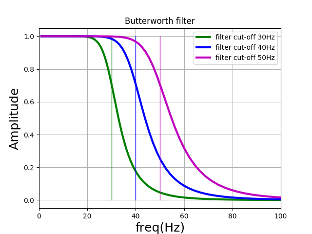
Figure 1: Illustration of the appearance of the Butterworth filter for various cutoff frequencies
3.6. Keyword PAS_INST#
♦ PAS_INST = dt [R]
No time for seismic signals. This value is used to determine the cutoff frequency for simulations by the formula \(F=1/(2\mathit{dt})\) (Shannon). Care must be taken to ensure that the cutoff frequency is large enough to properly model the phenomenon.
3.7. Keyword FREQ_PENTE#
◊ FREQ_PENTE = fp [R]
Slope for the evolution of the central frequency [\(\mathit{Hz}/s\)]: \(f(t)={f}_{0}+{f}_{p}({t}_{0}-t)\), where \({t}_{0}\) is the reference moment and \({f}_{0}\) is the central frequency at this time. In GENE_ACCE_SEISME, the reference moment is chosen as the moment in the middle of the strong phase: \({t}_{0}=\mathrm{0.5TSM}+{t}_{\mathit{ini}}\). Constant values are taken before and after the strong phase (it is advisable to consult R4.05.05 for more details). It is observed that, in general, the fundamental frequency decreases over time. In this case, you must give a negative slope: \({f}_{p}<0\). The code stops in error if function \(f(t)\) produces negative center frequencies over the duration of the strong phase. If FREQ_PENTE is not entered, then we take a constant fundamental frequency equal to \({f}_{0}\). This must be entered for option DSP, in the case of SPEC_UNIQUE, SPEC_MEDIANE or SPEC_FRACTILE, in the case of, or, the central frequency of the process is deduced from the target response spectrum.
Note:
If you don’t fill in FREQ_PENTE and if you choose a constant modulation function, you get a stationary process. This process corresponds to the DSP of classical Kanai-Tajimi (but filtered at low frequencies) .
3.8. Keyword NB_TIRAGE#
◊ NB_TIRAGE = Nbt [I]
The number of signals to be simulated. The default is \(1\).
3.9. Keyword INIT_ALEA#
◊ INIT_ALEA = ni [I]
If the keyword INIT_ALEA is entered, the seed of random sequences is initialized with this value. Two consecutive calculations with the same initialization then produce the same seismic signals. If the keyword is not entered, then the seed used is displayed in the message file.
3.10. Keyword COEF_CORR#
◊ COEF_CORR = rho [R]
This keyword makes it possible to specify a correlation coefficient for the generation of correlated signals. The correlation coefficient can take values between -1 and +1: \(-1<\mathit{rho}<1\).
If COEF_CORR is entered, then pairs of correlated signals are simulated, with correlation coefficient rho. These signals can represent the two components of correlated horizontal seismic signals or else time loads for multi-support studies.
In the TABLE_FONCTION output of the operator, the two components are identified by “NOM_PARA” which is equal to “ACCE1” for the first and “ACCE2” for the second signal.
3.11. Keyword RATIO_HV#
◊ RATIO_HV = ratio [R]
If RATIO_HV and COEF_CORR are both entered, then 3D signals are generated with correlated horizontal components (defined by the correlation coefficient rho, which may be zero) and a vertical component that is not correlated to the other two, but to which the horizontal/vertical ratio entered by RATIO_HV applies. This ratio is often taken to be equal to \(\frac{3}{2}\) but any other value greater than zero can be chosen. In the TABLE_FONCTION output of the operator, the three components are identified by “NOM_PARA” which is equal to “ACCE1” and “ACCE2” for the horizontal signals and “ACCE3” for the vertical component.
Note:
RATIO_HV is only available for option SPEC_FRACTILE and if COEF_CORR is specified. In other cases, it is sufficient to generate vertical signals by an independent call to GENE_ACCE_SEISME and by giving the target spectrum or the parameters of DSP for the vertical component.
3.12. Keyword factor MATR_COHE#
This keyword factor must be filled in if one wishes to generate spatial seismic fields. This is useful for doing a temporal study with seismic excitation that varies in space or of a multi-support type. The coherence function defines the spatial correlation of seismic movement. It is then necessary to enter the type of coherence function and, if applicable, the associated parameters. More details on this consistency function can be found in the documentation for operator DYNA_ISS_VARI [U4.53.31].
In operator output TABLE_FONCTION, signals are listed by their node name, for example NOEUD = N1.
3.12.1. Operand MAILLAGE#
♦ MAILLAGE = mail [mesh_sdaster]


Modeling mesh.
3.12.2. Operand GROUP_NO_INTERF#
♦ GROUP_NO_INTERF = gni [grno]
With this keyword, we define the group of nodes for which we want to generate a space-time seismic field.
3.12.3. Operand TYPE#
♦ TYPE = consistency model [txt]
We can choose between the coherence function of Mita & Luco (MITA_LUCO) or those of Abrahamson (ABRAHAMSON, ABRA_ROCHER, ABRA_SOLMOYEN).
If we choose MITA_LUCO, then we must also enter VITE_ONDE. The PARA_ALPHA parameter is optional, by default we take alpha = 0.1.
3.12.4. Operands VITE_ONDE and PARA_ALPHA#
♦ VITE_ONDE = wave_speed, [R]
◊ PARA_ALPHA =/0.1 [DEFAUT]
/alpha, [R]
A detailed description of these parameters can be found in [U4.53.31].
3.13. Keyword factor PHASE#
This keyword factor must be filled in if it is desired to generate a set of seismic signals taking into account the phase shift due to wave propagation. The arrival times of the signals are calculated according to the coordinates of the nodes of the mesh, and in relation to a reference point.
In operator output TABLE_FONCTION, signals are listed by their node name, for example NOEUD = N1.
3.13.1. Operand MAILLAGE#
♦ MAILLAGE = mail [mesh_sdaster]


Modeling mesh.
3.13.2. Operand GROUP_NO_INTERF#
♦ GROUP_NO_INTERF = gni [grno]
With this keyword, we define the group of nodes for which we want to generate a space-time seismic field.
3.13.3. Operand VITE_ONDE#
♦ VITE_ONDE = wave_speed, [R]
The speed of propagation of the wave.
3.13.4. Operand DIRECTION#
♦ DIRECTION = dir, [R]
The direction of propagation of the wave (directional vector: 3 values).
3.13.5. Operand COOR_REFE#
◊ COOR_REFE = crefe [R]
This keyword is optional. It allows you to enter the coordinates (3D) of a reference point for calculating the phase shift (wave arrival time). By default, we identify the mesh node that sees the wave first.
3.14. Keyword PESANTEUR#
♦ PESANTEUR = g [R]
In general, we take PESANTEUR =9.81 (\(m\mathrm{/}{s}^{2}\)) (cf. also §3.8.2). In this case, you must enter ACCE_MAX (PGA), and ECART_TYPE or, if applicable, the target spectrum (SPEC_OSCI) in \(g\). This normalization quantity is also used to calculate the Arias intensity. For example, giving ACCE_MAX = 0.2 corresponds to a PGA of \(\mathrm{0.2g}\) with \(g\mathrm{=}\mathrm{9.81m}\mathrm{/}{s}^{2}\). The accelerograms generated will then be accelerations in \(m/{s}^{2}\).
3.15. Keyword factor DSP#
The earthquake is modelled by a stochastic process that is not stationary. The evolving power spectral densities (DSP) make it possible to take into account a phenomenon that is not stationary in amplitude and frequency content such as an earthquake. The variation of the amplitude is taken into account by a modulation function while the evolution of the frequency content is modeled by the evolutionary Kanai-Tajimi DSP. Kanai-Tajimi’s DSP is also filtered in order to remove frequency content at very low frequencies that can lead to digital problems (non-zero drifts for integrated signals).
The parameters related to the variation of the amplitude are the Arias intensity, the duration of the strong phase and the moment of onset of the strong phase. The parameters related to DSP and the evolution of the frequency content are the damping and the fundamental frequency of the DSP of Kanai-Tajimi as well as the slope describing the evolution of this last one over time. These parameters can be determined from a given acelerogram, a SRO (oscillator response spectrum) or by using data available in the literature. In addition, since the model is parameterized, it is possible to take into account the variability and uncertainty of these parameters using random draws.
The simulation algorithm and the model are described in more detail in the reference documentation [R4.06.04].
3.15.1. Operands AMOR_REDUIT, FREQ_FOND#
♦ AMOR_REDUIT = friend [R]
Value of the critical damping ratio of Kanai-Tajimi’s DSP.
♦ FREQ_FOND = f0 [R]
The center frequency of Kanai-Tajimi’s DSP is the frequency where the most energy is concentrated.
3.16. Keywords factors SPEC_MEDIANE, SPEC_MOYENNE, SPEC_UNIQUE, and SPEC_FRACTILE#
This keyword factor makes it possible to fill in the data of a SRO target in order to generate seismic signals in accordance with the SRO target. It is then necessary to determine a DSP « compatible » with the data of the SRO target. There are several options:
SPEC_UNIQUE: Generation of a seismic signal whose SRO is very close to the SRO target: iterations must be carried out to best adjust the spectral content of the signal. If several signals are requested (NB_TIRAGE), then the adjustment is made per generated signal.
SPEC_MOYENNE, SPEC_MEDIANE: Generation of \(\mathrm{Nbt}\) signals whose median/medium spectrum respects the target. If the SRO target is a physical spectrum, then all the signals generated generally have a median SRO close to the target. However, we can do iterations to improve the adjustment of SRO, either in median (SPEC_MEDIANE) or average (SPEC_MOYENNE). If you don’t do any iterations (NB_ITER not specified) to improve the fit, then both options produce the same result.
SPEC_FRACTILE: Generation of :math:`mathit{Nbt}` signals whose median spectrum and the single-sigma spectrum respect the target. This is a « *best-estimate » method for studies. The signals generated have a variability close to that of the real signals available in the databases, in particular with regard to the variability between the realizations (record-to-record variability). To do this, it is necessary to fill in the median spectrum as well as the spectrum at one sigma. The median spectrum as well as the spectrum at one sigma are generally provided by attenuation laws.
3.16.1. Operand SPEC_OSCI#
♦ SPEC_OSCI = spec_target
Here we enter the SRO target in the form of a function with frequencies on the x-axis and the spectral accelerations on the x-axis (the latter must be normalized according to PESANTEUR). You can use DEFI_FONCTION to build it. If option SPECTRE_FRACTILE was chosen, then this spectrum must correspond to the median spectrum (as defined by attenuation laws).
3.16.2. Operand SPEC_1_SIGMA#
♦ SPEC_1_SIGMA = spec_target
Mandatory keyword for option SPEC_FRACTILE. Here, we enter the SRO to a target sigma in the form of a function with the frequencies on the x-axis and the spectral accelerations on the y-axis (the latter must be normalized according to PESANTEUR). You can use DEFI_FONCTION to build it. The spectrum at one sigma is, for example, provided by attenuation laws that assume a log-normal distribution of spectral accelerations and therefore of SRO values. This implies that SRO at one sigma corresponds to the 84% fractile of SRO. It is recommended to consult the reference documentation [R4.05.05] for more details on this modeling.
3.16.3. Operand AMOR_REDUIT#
♦ AMOR_REDUIT = friend [R]

 Depreciation value reduced by SRO entered under SPEC_OSCI.
3.16.4. Operands ERRE_ZPA, ERRE_RMS, and ERRE_MAX#
◊ ERRE_MAX = (cmax, emax) [R]
◊ ERRE_ZPA = (capa, ezpa) [R]

◊ ERRE_RMS = (crms, erms) [R]


These keywords are optional, you can enter the weighting coefficients as well as the maximum error desired by the user for the three adjustment criteria: maximum error on the frequency band, error on the ZPA (zero period acceleration) and error RMS. It is possible to enter a weighting coefficient (cmax, czpa, crms) but no maximum target error (emax, ezpa, erms). On the other hand, you must fill in the three weightings together. The calculated error is the relative error, namely the difference between the value of the realized spectrum and the value of the target spectrum divided by the value of the target spectrum. If the maximum error desired (emax, ezpa, erms). If one of the errors is greater than the value entered, an alarm is issued. The weighting coefficients are used to determine a weighted multi-objective error for each iteration. This criterion is used to choose, among the results of the iterations, the accelerogram (or the accelerograms) at the output of the calculation that best meet the criterion (it is not always the last iteration).
3.16.5. Operand NB_ITER#
◊ NB_ITER = number [I]
The number of iterations is entered to improve the adjustment of the accelerogram to the target spectrum (SRO). This keyword is optional: by default, we do not iterate. With option SPEC_FRACTILE, you can’t iterate.
3.16.6. Operand METHODE#
◊ METHODE = /” HARMO “[DEFAUT]
This optional keyword allows you to choose the method for calculating response spectra. These are the same methods that are available for calculating SRO with CALC_FONCTION [U4.32.04]. By default, we use the “HARMO” method. The response spectrum is then obtained by successive harmonic calculations (for various natural oscillator frequencies) through a FFT/IFFT of the input signal. The “NIGAM” method is detailed in document [R5.05.01].
3.16.7. Operand FREQ_PAS#
◊ FREQ_PAS = fpas [R]
- 3.6
With this optional keyword, you can choose the SRO discretization step used to determine which DSP is compatible. The SRO values entered via SPEC_OSCI are then interpolated to obtain the desired discretization step fpas. By default, we take the same frequency step as that used to generate the signals. The latter is deduced from the cutoff frequency and the number of points NB_POIN, cf. §.
3.17. Keyword factor MODULATION#
The parameters of the modulation functions GAMMA and of Jennings & Housner (JENNINGS_HOUSNER), are identified so that the mean TSM strong phase of the signals corresponds to that given. For a CONSTANTE modulation (no modulation), the duration of the simulated signals corresponds to TSM. We use the definition based on Arias’s intensity. We note \(\mathit{TSM}\mathrm{=}{T}_{2}\mathrm{-}{T}_{1}\) where \({T}_{1}\) and \({T}_{2}\) are respectively the moments of time when 5% and 95% of the Arias intensity (the total energy) are achieved. Moment \({T}_{1}\) corresponds to the start of the strong \({t}_{\mathit{ini}}\) phase.
If NB_POINest given for Gamma and Jennings & Housner modulations, then the total duration of the signals corresponds to (NB_POIN -1) * PAS_INST.
3.17.1. Operand TYPE#
♦ TYPE =/'JENNINGS_HOUSNER' [TXM]
/”GAMMA” /”CONSTANT”
Definition of the type of modulation (cf. also [R4.05.05]).
Type CONSTANT modulation corresponds to a signal without amplitude modulation. If we also assume that the fundamental frequency of DSP is constant, then we are back to a stationary process.
3.17.2. Operands INT_ARIAS, ACCE_MAX, ECART_TYPE#
If you have chosen option DSP, then you must enter one of the three parameters Arias intensity, PGA (maximum acceleration on the ground) or standard deviation to define the energy contained in the signals. If one of the three key words factor SPEC_UNIQUE, SPEC_MEDIANE, or SPEC_FRACTILE has been chosen, then this information is already contained in the target spectrum.
◊ INT_ARIAS = arias [R]


Average Arias intensity: :math:`\mathit{Arias}\mathrm{=}E(\frac{\pi }{2g}{\mathrm{\int }}_{0}^{\mathrm{\infty }}{X}^{2}(t)\mathit{dt})` with :math:`X` the process modeling seismic movement (acce) and :math:`g` is gravity.

 ◊ ACCE_MAX = PGA [R]
Maximum acceleration on the ground (PGA). This value is associated with the median maximum of the signals to be generated. The corresponding standard deviation is determined from the peak factor and for the strong phase TSM.
You must enter ACCE_MAX (PGA) in \(g\). The value of \(g\) must be entered using the PESANTEUR keyword. So ACCE_MAX = 0.2 corresponds to a PGA of \(\mathrm{0.2g}\) with \(g\mathrm{=}\mathrm{9.81m}\mathrm{/}{s}^{2}\). The accelerograms generated will then be accelerations in \(m\mathrm{/}{s}^{2}\).
◊ ECART_TYPE = ect [R]

Standard deviation of the underlying stationary stochastic process. Amplitude modulation (GAMMAou JENNINGS_HOUSNER) is then applied.

You must enter ECART_TYPE in :math:`g` (also enter above). The value of :math:`g` must be entered using the PESANTEUR keyword. We have to take PESANTEUR =9.81 (:math:`m\mathrm{/}{s}^{2}`) to get accelerations in :math:`m\mathrm{/}{s}^{2}`.
3.17.3. Operand INST_INIT#
♦ /◊ INST_INIT = t_ini [R]
Instant of start of the strong phase in the case of the modulation function GAMMA.
The parameters of the modulation function GAMMA are identified (by least squares) so that \(\mathit{TSM}\) and \({t}_{\mathit{ini}}\) are respected.
3.18. Operand INFO#
◊ INFO =
/1: no printing.
/2: printing information relating to the model and discretization (signal processing).
3.19. Operand TITRE#
◊ TITRE = title
title is the title of the calculation to be printed at the top of the results [U4.03.01].