3. Operands#

3.1. Operands INST_INIT/INST_FIN#

◊ INST_INIT = ii

First value of the parameter for which the signals will be used to calculate the interspectral matrix (initial instant).

♦ INST_FIN = if

Last value of the parameter for which the signals will be used to calculate the interspectral matrix (final instant).

Note:

The functions will be calculated using the interpolation mode associated with them. To avoid discretization problems, it is recommended that the functions have an authorized linear interpolation.

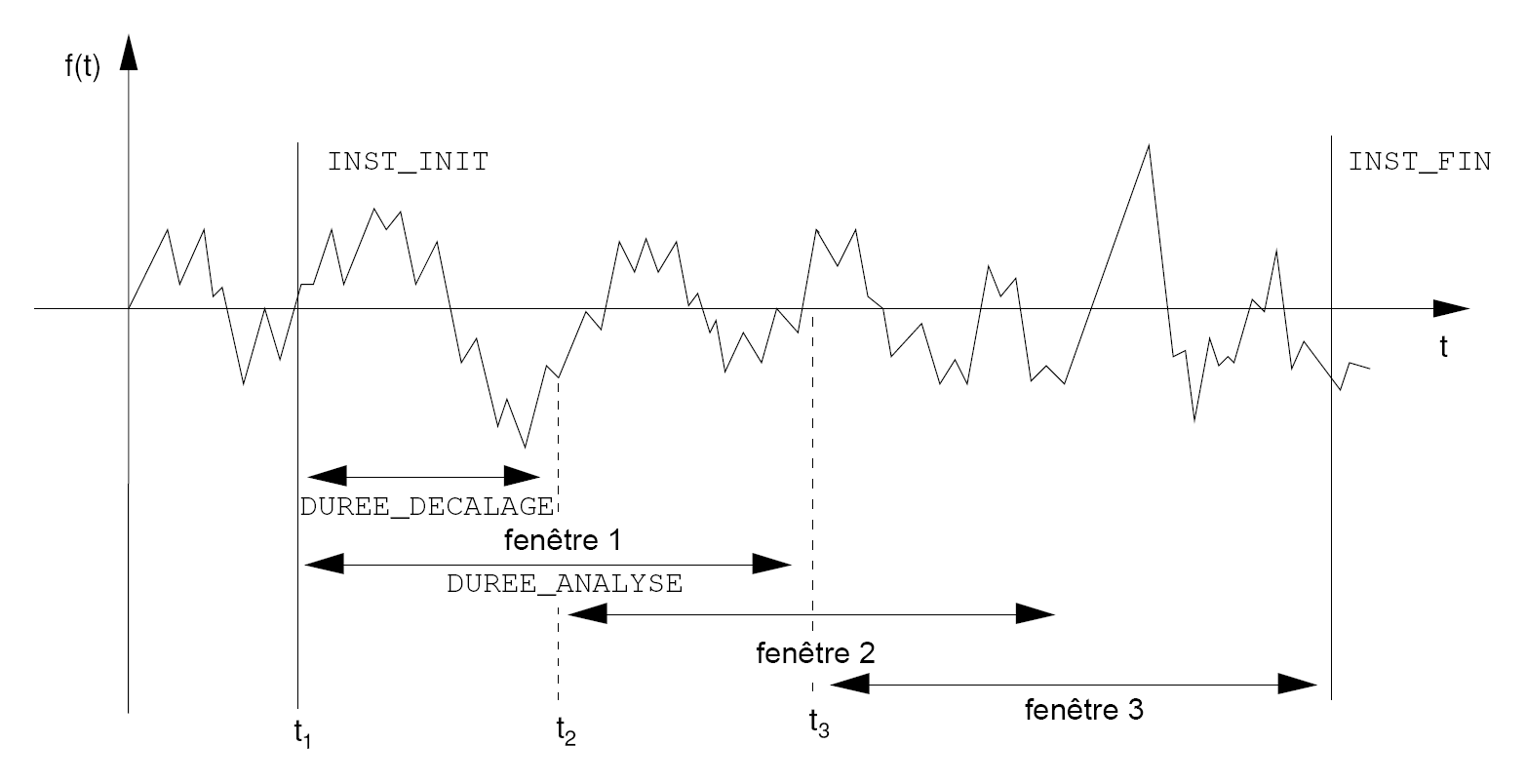
Figure 3.1-a: Analysis and calculation on 3 windows with overlay

3.2. Operands DUREE_ANALYSE/DUREE_DECALAGE#

◊ DUREE_ANALYSE = da

The functions will be divided into several windows of analysis duration da. For each of these windows an interspectral matrix is calculated. The interspectral matrix resulting from the operator will be the arithmetic mean of the calculated matrices.

◊ DUREE_DECALAGE = dd

Allows, when dividing functions according to the analysis duration into windows, to shift each window relative to each other by a duration dd. If \({t}_{k}\) is the initial instant of the \({k}^{\text{ième}}\) window, the initial instant of the \({(k+1)}^{\text{ième}}\) window will be \({t}_{k}\) +dd.

Let \(x[k]\) and \(y[k]\) be two discrete time signals and \({x}_{p}[k]\) and \({y}_{p}[k]\) the respective time windows obtained by chopping.

If \(X[k]\) and \(Y[k]\) designate their discrete FOURIER transforms, then the interspectral matrix is written as [bia1]:

\(S[k]\text{vaut}(\begin{array}{cc}{S}_{\mathrm{xx}}[k]& {S}_{\mathrm{xy}}[k]\\ {S}_{\mathrm{xy}}^{\text{*}}[k]& {S}_{\mathrm{yy}}[k]\end{array})\)

where

\({S}_{\mathrm{xx}}[k]=\frac{1}{\mathrm{p.n}\Delta t}\sum _{i=1}^{p}{X}_{p}[k]\mathrm{.}{X}_{p}^{\text{*}}[k]\)

\({S}_{\mathrm{xy}}[k]=\frac{1}{\mathrm{p.n}\Delta t}\sum _{i=1}^{p}{X}_{p}[k]\mathrm{.}{Y}_{p}^{\text{*}}[k]\)

where \(n\) is the number of points per block,

\(p\) is the number of blocks.

Attention:

This averaging, which is perfectly adapted to the « real » signals (results of a measurement), is not suitable without precaution for functions close to a sine (the averaging frequency must be much higher than the signal frequency).

Note:

If the signals processed come from the operator GENE_FONC_ALEA possibly via the calculation of a dynamic response (operator DYNA_TRAN_MODAL for example), then it is advisable to process each of the draws of GENE_FONC_ALEA independently. In this case, you must choose analysis and lag times equal to the duration of each of the draws of GENE_FONC_ALEA (cf. GENE_FONC_ALEA [U4.36.05] ) .

3.3. Operand NB_POIN#

♦ NB_POIN = no

Number of parameter points for an analysis period. For each point the functions will be calculated according to the type of interpolation and extension defined. The number of points must be a power of 2 (fast Fourier transform calculation).

Note:

If the signals consist of a sufficient number (power of two) of points with a constant step, it is preferable to choose this number to avoid interpolations that can generate artifacts. In particular, if the signals processed come from the operator GENE_FONC_ALEA possibly via the calculation of a dynamic response (operator DYNA_TRAN_MODAL for example), this number will correspond to twice the number of points entered in GENE_FONC_ALEA keyword NB_POIN or obtained by INFO =2 in GENE_FONC_ALEA (cf. GENE_FONC_ALEA [U4.36.05]) .

3.4. Operand FONCTION#

♦ FONCTION =

List of the names of functions (time signals) of a function-type concept, whose interspectral matrix we want to calculate.

3.5. Operand TITRE#

◊ TITRE =

title is the title of the interspectrum concept to be printed at the top of the results [U4.03.01].

3.6. Operand INFO#

◊ INFO =

Specify the print options on file MESSAGE.

1	prints the initial frequency, the final frequency, and the frequency step.
2	like 1plus for each autospectrum and interspectrum, a convergence criterion according to the number of random draws. (a random draw corresponds to an analysis window).