4. Examples

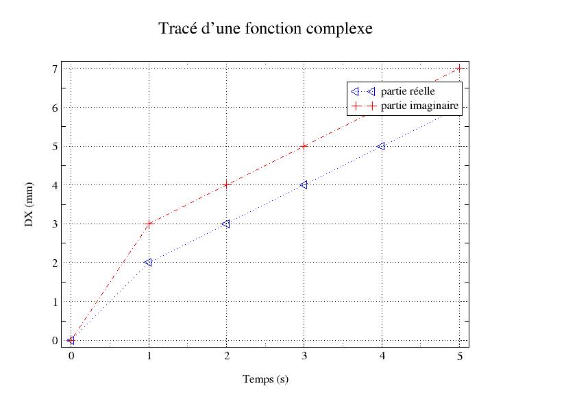
4.1. Curve representing a complex function

fc = DEFI_FONCTION (NOM_PARA =” INST “, NOM_RESU =”DX”,

VALE_C =( 0., 0., 0., 0., 0., 1., 2., 3. ,

2., 3., 4., 4., 4., 5. ,

4., 5., 6., 5., 5., 5., 5., 7.),)

IMPR_FONCTION (

UNITE = 24,

FORMAT = “XMGRACE”,

PILOTE = “POSTSCRIPT”,

LEGENDE_X = “Time (s) “,

LEGENDE_Y = “DX (mm) “,

COURBE = (

_F (FONCTION = fc,

PARTIE = “REEL”,

COULEUR = 4,

STYLE = 2,

MARQUEUR = 5,

LEGENDE = “real game”,),

_F (FONCTION = fc,

PARTIE = “IMAG”,

COULEUR = 2,

STYLE = 5,

MARQUEUR = 8,

LEGENDE = “imaginary part”,),

),

TITRE = « Plot of a complex function »,

)

4.2. Parametric curve

lt = DEFI_LIST_REEL (DEBUT = 0., INTERVALLE =_F (JUSQU_A =10., PAS =0.01),)

fx = FORMULE (NOM_PARA =”t”,

VALE = « 2. *cos (t) - cos (2.*t) « « ,)

CardioX= CALC_FONC_INTERP (

FONCTION = fx,

LIST_PARA = lt,)

fy = FORMULE (NOM_PARA =”t”,

VALE = « 2. *sin (t) - sin (2.*t) « « ,)

CardioY= CALC_FONC_INTERP (

FONCTION = fy,

LIST_PARA = lt,)

IMPR_FONCTION (

UNITE = 27,

FORMAT = “XMGRACE”,

TITRE = “Cardioid”,

COURBE = (

_F (FONC_X = CardioX,

FONC_Y = CardioY,),

),

)

We thus obtain a file that can be viewed in xmgrace:

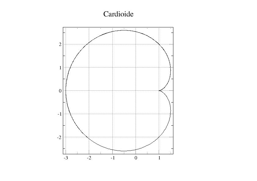
Additional formatting in xmgrace: Plot/Graph apparance menu, type*fixed* (square grid), and remove the legend by unchecking the*Display legend* box.

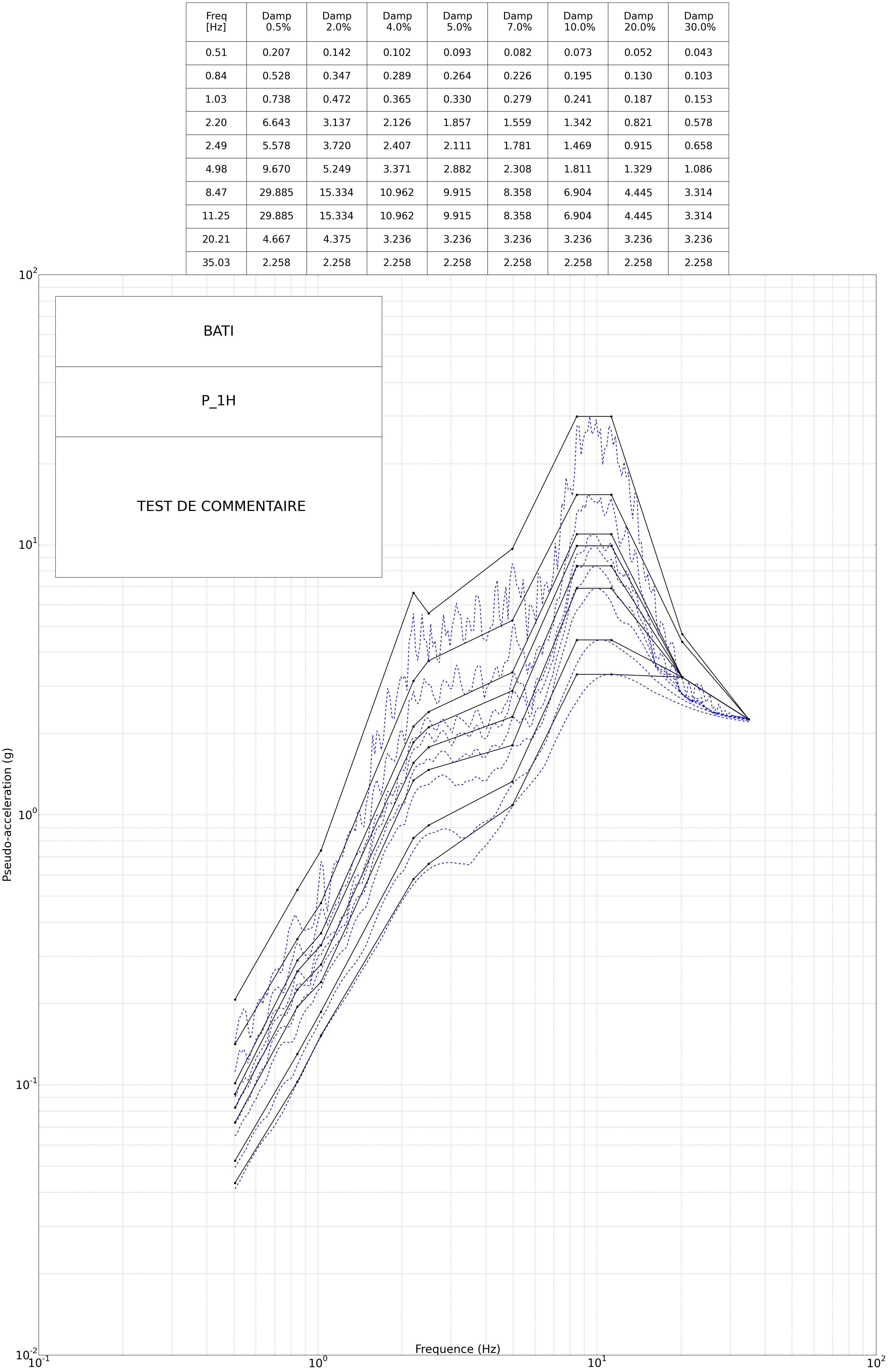
4.3. Tablecloth and smooth tablecloth

A next.png file is thus obtained.