3. Operands#
3.1. Keyword DERIVE#
/DERIVE =
We derive function \(f(t)\).
Name of the function you want to derive.
Does not apply to tablecloth-type concepts.
Name of the METHODE you want to use: the only method available is currently DIFF_CENTREE (by default).
Remarks:
See keyword INTEGRE.
3.2. Keyword INTEGRE#
/INTEGRE =
We integrate the \(f(t)\) function.
Integration constant, by default 0.
Name of the function you want to integrate.
Does not apply to tablecloth-type concepts.
Name of the METHODE you want to use.
Two methods are available: the “TRAPEZE” method (by default) and the “SIMPSON” method.
The integral is accurate for piecewise linear functions as input. The error committed in relation to the integral of the function that we discretized is in \(o(1\mathrm{/}{n}^{2})\) for functions of classes \({C}^{2}\).
The Simpson method is accurate for polynomials with a degree less than or equal to 3. The error is in \(o(1\mathrm{/}{n}^{4})\) for functions of classes \({C}^{4}\).
For random, very hectic functions, such as accelerographs, it is recommended to use the trapezius method.
On the other hand, when function \(f(t)\) (before discretization) is sufficiently regular, the Simpson method is much more accurate.
Remarks:
For INTEGREcomme for DERIVE, the NOM_PARAde function produced is unchanged. On the other hand, the NOM_RESUpeut be modified in the following cases: for derivation, DEPLdevient VITE, VITEdevient * ACCE; for integration, ACCEdevient * VITE, * , * , * VITE * **; for integration, * ** * , , , * , * ** * ** . DEPL The user always has the option of modifying it by the keyword of the same name in CALC_FONCTION.
Regarding extensions, the function produced has, by default, extensions * EXCLUà left and right regardless of those of the starting function. So do not expect a linear extension to become constant in the derived function… Again, the user is in control of his extensions for the function produced by the keywords PROL_DROITE and and PROL_GAUCHE.
3.3. Keyword INVERSE#
/INVERSE =
We reverse function \(f(t)\).
Name of the function you want to invert, it must be bijective (strictly increasing or strictly decreasing).
Does not apply to tablecloth-type concepts.
Note:
Parameter labels are not reversed! It is up to the user to assign the correct values with the keywords NOM_PARAet NOM_RESU. By default, the NOM_PARAest unchanged and NOM_RESUest assigned to “ TOUTRESU “ .
Interpolation modes are swapped: e.g. (“LIN”, “ LOG “) becomes (” LOG “,” LIN “) .
The extensions EXCLUet * LINEAIREsont unchanged. In contrast, an extension CONSTANTest changed to EXCLU.
3.4. Keyword ABS#
/ABS =
Provides the absolute value of a function or table.
Name of the function whose absolute value we want.
Note:
The parameters (extensions, interpolations, * NOM_PARAet NOM_RESU) of the function produced are the same as those of the original function.
Except for the extension LINEAIRE: systematically changed to EXCLUpar precaution. Indeed, the linear extension of a decreasing function to the right leads to negative values for sufficiently large abscissa values: responsibility is therefore left to the user to assign himself PROL_DROITE =” LINEAIRE “(and respectively to the left) .
3.5. Keyword ENVELOPPE#
/ENVELOPPE =
Calculation of the envelope of several functions.
This operation is available on operands of a function or layer nature.
3.5.1. Operand FONCTION#
♦ FONCTION = f
List of functions or sheets whose envelope we are looking for.
3.5.2. Operand CRITERE#
◊ CRITERE =
/”SUP”
We’re looking for the top envelope.
/”INF”
We’re looking for the lower envelope.
Notes for finding the envelope:
the functions must all be of the same nature (function or table),
Case of simple functions: for extensions, interpolations, * NOM_PARA * and NOM_RESU, the parameters of the first of the functions in the list are retained. The abscissa support of the envelope function will be the meeting of the abscissa lists of all the functions.
Case of tablecloths: the parameters (extensions, interpolations, , interpolations, NOM_PARA, NOM_RESU, NOM_PARA_FONC) must imperatively be identical between the sheets provided. The x-axis supports (values of the parameters and x-axis of the functions of the layers) are homogenized in order to be able to calculate the envelope. The tablecloth produced will have this discretization as its abscissa.
3.6. Keyword FRACTILE#
/FRACTILE =
Calculating the fractile of several functions.
This operation is available on operands of a function or layer nature.
3.6.1. Operand FONCTION#
♦ FONCTION = f
List of functions or layers whose fractile we want to calculate.
3.6.2. Operand FRACT#
♦ FRACT = fract
Quantile value to be calculated. By default fract = 1, the fractile is then the upper envelope.
3.7. Keyword MOYENNE#
/MOYENNE =
Calculation of the average of several functions.
This operation is available on operands of a function or layer nature.
3.8. Keyword COHERENCE#
/COHERENCE =
Calculation of the coherence function of time signals.
The coherence function depends on the distance between two measurement points and on the frequency. It expresses the correlation between the two signals, measured at a distance \(d\), as a function of frequency. The complex coherence function is evaluated in the frequency domain, using spectral densities (DSP). The operator returns the real part of the complex coherence, which corresponds to the « unlagged coherency » or the « plane wave coherency » in the case of a plane wave.
The time signals must have the same discretization (same time step \(\mathit{dt}\) and same duration \(T\)). The user must provide two sheets that respectively contain the signals to stations 1 and 2, separated from \(d\). The signals in each sheet are parameterized by NUME_ORDRE (1,2,3,..) and then matched to calculate the consistencies and take the average.
3.8.1. Operands NAPPE_1 and NAPPE_2#
♦ NAPPE_1 = tablecloth1
Tablecloth containing N functions measured at station 1. The functions of the tablecloth must be numbered from 1 to N by NOM_PARA = “NUME_ORDRE”.
♦ NAPPE_2 = tablecloth2
Tablecloth containing N functions measured at station 2. The functions of the tablecloth must be numbered from 1 to N by NOM_PARA = “NUME_ORDRE”.
3.8.2. Operand FREQ_COUP#
◊ FREQ_COUP = fc
Cutoff frequency for plotting coherence functions. The cutoff frequency should be less than \(\frac{1}{2\times \mathit{dt}}\), where \(\mathit{dt}\) is the time step for time signals. For the evaluation of coherence functions, the cutoff frequency is always determined by the time step of the time signals. If FREQ_COUP is entered, then the consistency function is cut to \(\mathit{fc}\) before rendering.
3.8.3. Operand NB_FREQ_LISS#
◊ NB_FREQ_LISS =/12 [default]

/NFL
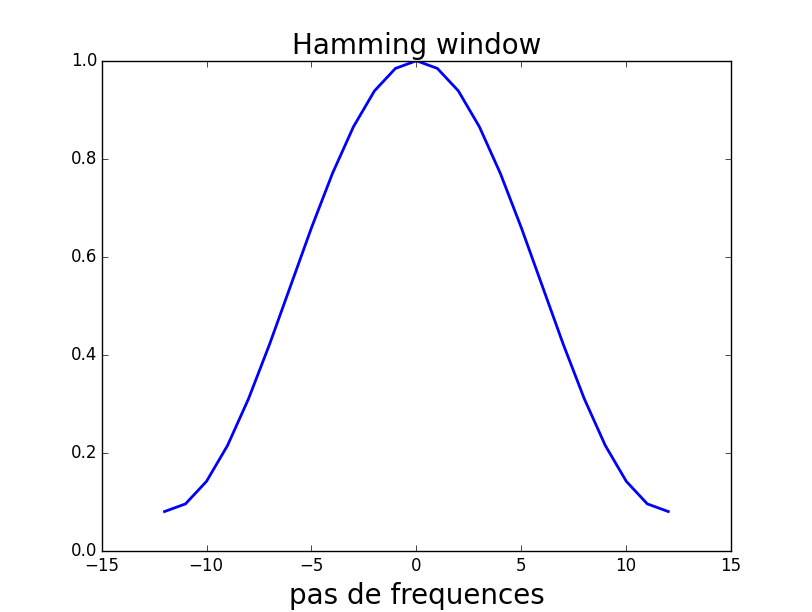
Number of frequency steps used for smoothing DSP per Hamming window. The Hamming window obtained with NB_FREQ_LISS = 12 is shown in the figure below.
3.8.4. Operands OPTION, BORNE_INF, and BORNE_SUP#
◊/OPTION =
Allows you to define whether the entire signal or only the strong phase is used to calculate the coherence function:
/”TOUT” [DEFAUT]
Time signals are used as they are.
/”DUREE_PHASE_FORTE”
The coherence function is evaluated for the duration of the strong phase only. The start and end times of the strong phase are calculated for the first signal only. The same time interval is then used for the other signals. In the case of an earthquake, this assumes that all records are from the same event. To assess the duration of the strong phase, the concept of Arias intensity is used. You must then fill in the lower and upper limits (cf. [U4.32.05]).
◊ BORNE_INF = /0.05

/binf,

◊ BORNE_SUP = /0.95

/bsup,
Boundaries limiting the Arias intensity portion defining the initial and final moments of the strong phase (between \(({b}_{\text{inf}})\text{\%}\) and \(({b}_{\text{sup}})\text{\%}\) of the Arias intensity) of the earthquake - same meaning as for INFO_FONCTION. By default, we take 5% and 95%.
3.9. Keyword COMB and operand LIST_PARA#
/COMB =
Real linear combination of several concepts of a function or sheet nature.
The name of the function to be combined.
Value of the coefficient.
◊ LIST_PARA = for
List of parameter values for which the combination of functions will be discretized. If this keyword is not filled in, a list by default is constructed by taking the union of the lists of the values of the parameters of each function.
Attention:
It is not a key word for the factor keyword COMB.
Notes for the combination:
See notes for the keyword ENVELOPPE
3.10. Keyword COMB_C and operand LIST_PARA#
/COMB_C =
Complex linear combination of several concepts of a function_c nature.
The name of the function to be combined. It can have complex or real values.
/COEF_R = r, /COEF_C = c,
Value of the multiplier coefficient, either in real form r or in complex form c.
◊ LIST_PARA = for
List of parameter values for which the combination of functions will be discretized. If this keyword is not filled in, a list by default is constructed by taking the union of the lists of the values of the parameters of each function.
Notes for the combination:
See notes for the keyword ENVELOPPE
3.11. Keyword MULT and operand LIST_PARA#
/MULT
Product of concepts of the same nature: function, function_c, or tablecloth.
Name of the function to be multiplied with the others.
LIST_PARA allows you to discretize the result function as for COMB.
3.12. Keyword COMPOSE#
Keyword factor used to calculate the compound of two functions \(F(G(t))\).
Does not apply to tablecloth-type concepts.
/COMPOSE =
f_resu (x) function
f_para (t) function
We check that the NOM_PARA of f_resu corresponds to the NOM_RESU of f_para.
3.13. Keyword ASSE#
/ASSE =
A factor keyword that allows you to create a real function by concatenating two tabulated real functions.
Does not apply to tablecloth-type concepts.
3.13.1. Operand FONCTION#
Functions to concatenate. Exactly two functions are expected.
3.13.2. Operand SURCHARGE#
/”GAUCHE”,
The discretization points of the created function are those of the set of the two functions, modulo the effects of overload.
If the areas of definition of the functions overlap, one of the functions imposes its points on the overlap zone and for extensions:
SURCHARGE =/”DROITE”: it is the function that has the largest xmax that is chosen,
SURCHARGE =/”GAUCHE”: the function with the lowest xmin is chosen.
3.13.3. Checks#
We check that all the functions have the same NOM_PARA, as well as the same interpolations.
3.14. Keyword EXTRACTION#
/EXTRACTION =
Keyword factor allowing to build from a complex function (type funct_c), a real function representing either the real part, or the imaginary part, or the module, or the phase of the complex function.
3.14.1. Operand FONCTION#
Complex function.
3.14.2. Operand PARTIE#
/ 'REEL'
|
: |
extracting the real part of f_c, |
/ 'IMAG'
|
: |
extracting the imaginary part of f_c, |
/ 'MODULE'
|
: |
extracting the module from f_c, |
/ 'PHASE'
|
: |
extraction of the phase (in degrees) of f_c. |
3.15. Keyword PUISSANCE#
This keyword makes it possible to build the nth power of a function or a set of functions provided in the form of a sheet.
♦ FONCTION = f
Name of the function f concerned (function or tablecloth type).
♦ EXPOSANT = n
The calculated result function will be \(x\to f{(x)}^{n}\). By default, \(n\mathrm{=}1\).
3.16. Keyword REGR_POLYNOMIALE#
This keyword calculates the polynomial regression of a function using the least squares method (using the numpy polyfit function).
♦ FONCTION = f
Name of the function f concerned (function type).
♦ DEGRE = n
Degree of the polynomial sought.
The keyword LIST_PARA can be used to tabulate the calculated polynomial. Otherwise, it is tabulated to the list of abscissa for the function f.
3.17. Keyword FFT#
/FFT =
The direct or inverse Fourier transform of a function is calculated (including by algorithm FFT).
♦ FONCTION = f
Name of the function on which the operation is performed.
If the NOM_PARA of the function is INST, then the direct FFT is calculated.
If the NOM_PARA of the function is FREQ, then the inverse FFT is calculated.
Does not apply to tablecloth-type concepts.
♦ METHODE =
Algorithm FFT is faster for samples whose length is a power of 2.
The “PROL_ZERO” method (by default) proposes to extend the input signal with zeros until we have a total number of samples which is the first power of 2 whose value is greater than the initial number of samples.
The “TRONCATURE” method will only consider the first samples whose total number is the greatest power of two whose value is less than the initial number of samples.
For example, on a signal with 601 values, the “PROL_ZERO” method will complete the signal to have 1024 samples, while the “TRONCATURE” method will only consider the first 512 moments.
If the input signal has a sample number that is a power of two, the two methods are obviously equivalent: the signal is taken into account without modifying it.
The “COMPLET” method makes it possible to take into account the entire input signal, regardless of the number of samples.
Note: in the case of a sample of length \(N\), whose time step would be \(\mathit{dt}\), the sample rate for FFT is \(1\mathrm{/}(\mathit{N.dt})\). On the other hand, the last frequency for which the discrete transform is calculated is not \(1\mathrm{/}\mathit{dt}\), but \((N\mathrm{-}1)\mathrm{/}(\mathit{N.dt})\).
♦ SYME =
A keyword that only applies to the inverse Fourier transform.
In the case where the full spectrum is provided, then the inverse transform is calculated directly using SYME = “OUI”. The methods” TRONCATURE “and” PROL_ZERO “are then not active.
If the (complex) spectrum supplied as input to the inverse FFT does not contain the folded part (associated with the negative frequencies of the spectrum), it is nevertheless possible to estimate a time signal having the same spectral content on the part associated with the positive frequencies. If we write \({X}_{k}\) the \(k\) th sample of the Fourier transform of a sample of length \(N\), then we have \({X}_{k}\mathrm{=}{X}_{(N\mathrm{-}k)}^{\text{*}}\), where \({()}^{\text{*}}\) corresponds to the conjugate complex. This information can be used to reconstruct a time signal while knowing only half of the spectrum. This operation is performed when you choose SYME = “NON”. The time signal is then reconstructed to obtain a time sample of even length. In theory, to reconstruct a time signal of length \(2\mathrm{\times }M\), the spectrum must satisfy certain conditions:
The spectrum must be of length \(M+1\),
The first point in the spectrum must be real,
The last point in the spectrum must be real.
If these conditions are not satisfied, then an approximate spectrum of odd length is constructed satisfying these conditions. If the initial spectrum is of even length, the last point is then reconstructed by extending the initial spectrum by interpolation. This reconstruction may introduce a slight bias when the spectral content of the sample is very significant at the last points of the spectrum.
The methods” TRONCATURE “and” PROL_ZERO “are still available for the opposite FFT. Be careful, however, with the use of the “TRONCATURE” method. If the number of truncated points is significant, then the results can be very significantly different.
3.18. Keyword INTERPOL_FFT#
/INTERPOL_FFT =
Interpolation of an accelerogram using the « zero padding » method. This method consists in calculating the Fourier transform of the initial signal, in completing the frequency signal obtained by new frequencies of zero value and then in calculating the inverse Fourier transform of this modified frequency signal. This feature uses the same algorithms as the FFT keyword. The method is necessarily “COMPLET” and SYME = “NON”.
It makes it possible not to add frequency content to the interpolated function.
♦ FONCTION = f
Name of the function on which the operation is performed.
NOM_PARA of the function is necessarily INST.
♦ PAS_INST =
Desired time increment for the interpolated signal. Should be smaller than the time increment of the function provided.
◊ PRECISION =
/prev
/0.01 [DEFAUT]
The actual time step obtained is often slightly different than that shown via PAS_INST. This operand defines the maximum desired difference between these two values, if it is exceeded, an alarm message is sent to warn the user.
3.19. Keyword CORR_ACCE#
/CORR_ACCE =
Keyword factor for correcting an accelerogram (accelerating seismic signal) so that the moving signal does not have a drift. The corrected accelerogram is returned to the output. The signal can then be integrated using standard methods (keyword INTEGRE of CALC_FONCTION). The quality of the result should be verified by verifying the absence of signal drift while traveling and by comparing the response spectra before and after modification.
3.19.1. Operand FONCTION#
♦ FONCTION = f
Actual accelerogram measured.
Does not apply to tablecloth-type concepts.
3.19.2. Operand METHODE#
♦ METHODE =
Name of the METHODE that you want to use to correct signals: correction by polynomials or by filtering in the frequency domain.
METHODE =” POLYNOME “
The drift of the signal is eliminated, calculated by linear smoothing in the sense of least squares over the entire signal. The corresponding relative speed drift is also suppressed.
◊ CORR_DEPL =
/”NON”
We don’t correct the relative displacement drift, it’s the default value.
/”OUI”
The drift of relative displacement is also eliminated. This option should be used with caution, as the value of the final displacement after the earthquake is not known a prima facie.
METHODE =” FILTRAGE “
The drift is eliminated by filtering (« high pass ») of the signal in the frequency domain. This filter is described in the R4.05.05 documentation (section 2.1).
◊ FREQ_FILTRE =
/en
/0.05 [DEFAUT]
It is necessary to choose the lowest frequency that makes it possible to obtain the expected effect, namely to eliminate the drift, without (too) altering the other properties of the signal. By default, the filter frequency is 0.05Hz. This value is generally well suited for seismic signals. This value can be reduced if the signal allows it or increased if a drift persists.
3.20. Keyword LISS_ENVELOP#
♦/NAPPE = n
Name of the input sheet (s) formed from the raw spectra associated with each damping level. The sheet therefore depends on the frequency and damping parameters.
/TABLE = tab
Name of the input table or tables formed from the raw spectra associated with each damping level. In the expected format, the first column contains the frequency values, each of the following columns contains the acceleration value associated with the frequency for a given damping level. Depreciation values are given by LIST_AMOR.
/FONCTION = n
Name of the function formed from the raw spectrum associated with a level of damping.
♦ OPTION =
/”CONCEPTION” The first step consists in creating an envelope on the spectra provided. In a second step, the spectrum obtained is smoothed according to the number of smoothed points requested NB_FREQ_LISS.
/”VERIFICATION”
The first step consists in smoothing each spectrum provided according to the number of points requested. Then, each spectrum is broadened according to the coefficients provided in ELARG. In a third step, the envelope of the expanded spectra is calculated. Finally, the last step smoothes the spectrum obtained as a function of the number of smoothed points requested.
◊ NB_FREQ_LISS
Number of frequencies desired for the smoothed spectrum. In the case of the “CONCEPTION” option, only one value is provided. For the “VERIFICATION” option, you can provide two values that will be applied to the first step and to the fourth step.
◊ FREQ_MIN and FREQ_MAX
Frequency definition range of the smoothed spectrum.
The frequencies mentioned under FREQ_MIN and FREQ_MAX must be selected from the discretization frequencies of the raw spectrum.
By default, the full spectrum is considered.
◊ ELARG

     Enlargement covers an entire spectrum. You must provide as many values as there are numbers of tables or tables.

     For each frequency Fi of the raw spectrum, two new frequency values are defined such as:
\({F}^{\text{-}}={F}_{i}(1-{\tau }_{g})\) with \(0<{\tau }_{g}<1\);
\({F}^{\text{+}}={F}_{i}(1+{\tau }_{d})\) with \(0<{\tau }_{d}<1\).
The parameters \({\tau }_{g}\) and \({\tau }_{d}\) represent the amplitude of the frequency broadening and are equal to the value provided.
The values of the eccentric frequencies \({F}^{\text{-}}\) and \({F}^{\text{+}}\) do not correspond to the values \({F}_{i}\) in the raw spectrum definition list. We define \({F}_{j}\) and \({F}_{k}\) as follows:
\({F}_{j}\): value belonging to the list, immediately less than or equal to \({F}^{\text{-}}\),
\({F}_{k}\): value belonging to the list, immediately less than or equal to \({F}^{\text{+}}\).
For each frequency \({F}_{i}\), two coordinate points \(({F}_{j},{\gamma }_{i})\) and \(({F}_{k},{\gamma }_{i})\) are defined, where \({\gamma }_{i}\) represents the acceleration at frequency \({F}_{i}\). Two new spectra resulting from the shift of the raw spectrum on the frequency axis are therefore constructed. Then we calculate the envelope.
◊ LIST_FREQ
List of frequencies that you want to keep for the smoothed spectrum. The items in this list must be contained in the frequency values of the spectra taken as input.
◊ LIST_AMOR
List of depreciations that we want to associate with the various acceleration values from the table provided.
◊ ZPA
Value of the acceleration at high frequency that one wishes to impose for the smoothed spectrum.
By default, this is the spectrum value that is least damped at the highest frequency.
An example of application is proposed in test case ZZZZ100E.
3.21. Keyword SPEC_OSCI#
/SPEC_OSCI =
When METHODE = “NIGAM” (default) or “HARMO” (cf. § 3.21.1), NATURE_FONC = “ACCE” (cf. § 3.21.2), the oscillator spectrum of an accelerogram [R4.05.03] given under the keyword FONCTION (cf. §) is calculated. 3.21.1
The oscillator spectrum can only be calculated using the functions of NOM_RESU = “ACCE” and NOM_PARA = “INST”.
For all \(i\) and all \(j\) we consider \({q}_{j}^{i}\) to be the solution of the differential equation:
\({\ddot{q}}_{j}^{i}+2{\mathrm{\xi }}_{j}{\mathrm{\omega }}_{i}{\dot{q}}_{j}^{i}+{\mathrm{\omega }}_{i}^{2}{q}_{j}^{i}=f(t)\)
with \({q}_{j}^{i}(0)={\dot{q}}_{j}^{i}(0)=f(0)\) and \({\mathrm{\omega }}_{i}=2\mathrm{\pi }{\mathrm{\phi }}_{i}\)
Product concept \(\mathit{fr}\) is a table (function with two variables) consisting of functions \(\left({\mathit{fr}}_{i},\mathrm{...},{\mathit{fr}}_{j},\mathrm{...}\right)\) with \({\mathit{fr}}_{j}\) function defined at points \({\mathrm{\omega }}_{i}\) with:
- math:
{mathit {fr}} _ {j} ({mathrm {omega}} _ {i}) =underset {tmathrm {in} D} {mathit {Max}} {mathit {Max}}}}left| {j} (t)mathit {defined}right}
By default for calculating the oscillator spectrum
For reduced depreciation, the values are considered to be:
the following 150 values are considered for frequencies in \(\mathit{Hz}\),
the first is at :math:`0.2\mathit{Hz}` and we deduce the following ones by the rule;

from the 2nd to the 57th: in steps of 0.05 Hz
58 65 0.075 Hz 66 79 0.10 Hz 80 103 0.125 Hz 104 131 0.25 Hz 132 137 0.5 Hz 138 141 1. hz 142 150 1.5 Hz
The cutoff frequency by default is therefore \(\mathrm{35,5}\mathit{Hz}\) (the user must check that this value is consistent with the frequency content of the input signal; if this is not the case, a list of suitable frequencies must be defined).
the spectrum is standardized according to the value of NORME.
When METHODE = “RICE” (cf. § 3.21.1), NATURE_FONC = “), =” DSP “(cf. § 3.21.2), the oscillator spectrum equivalent to a power spectral density (DSP) [R4.05.03] is calculated under the keyword FONCTION (cf. §). 3.21.1 The function should be NOM_PARA = “FREQ”.
3.21.1. Operand FONCTION#
Name of the function on which the operation is performed.
Does not apply to tablecloth-type concepts.
3.21.2. Operands NATURE/NATURE_FONC#
Nature of the size of the tablecloth created by command CALC_FONCTION.
ACCE |
Absolute pseudo-acceleration spectrum |
\(\ddot{u}(t)={\mathrm{\omega }}_{i}^{2}u(t)\) |
VITE |
Relative pseudo-speed spectrum |
\(\dot{u}(t)={\mathrm{\omega }}_{i}u(t)\) |
DEPL |
Relative displacement spectrum |
\(u(t)\) |
/”DSP”
Nature of the function that is used to build the spectrum. The choice is imposed according to the method selected: “ACCE” (time signal) or “DSP” (accelerating power spectral density). This keyword allows you to override the NOM_RESU of the function specified under the FONCTION keyword when it is created by RECU_FONCTION [U4.32.03].
3.21.3. Operand METHODE#
Name of the METHODE that we want to use: the method by default, “NIGAM”, is detailed in the document [R5.05.01]. If we choose the “HARMO” method, then the response spectrum is obtained by successive harmonic calculations (for various natural oscillator frequencies) by going through a FFT/IFFT of the input signal. If we choose “RICE” then we determine the SRO equivalent for the data of a DSP.
3.21.4. Operand TYPE_RESU#
/”FONCTION”
By default, using SPEC_OSCI produces a tablecloth. If AMOR_REDUIT only contains damping, a sheet containing only one function is created. In this case, you can choose TYPE_RESU =” FONCTION “to return this function directly.
3.21.5. Operand AMOR_REDUIT#
Lam = \(\left({\mathrm{\xi }}_{1},\mathrm{...},{\mathrm{\xi }}_{i},\mathrm{...}\right)\)
List of reduced depreciations: example 0.01, 0.05,…
3.21.6. Operands FREQ/LIST_FREQ#
◊ FREQ = lfre
free = \(\left({\mathrm{\phi }}_{1},\mathrm{...},{\mathrm{\phi }}_{i},\mathrm{...}\right)\). List of frequencies.
◊ LIST_FREQ = lfreq
List of frequencies provided under a listr8 concept.
The frequencies must be strictly positive.
3.21.7. Operand NORME#
The oscillator spectrum will be normalized to the value r (value of the pseudo-acceleration), this value is recalled in the message file.
3.21.8. Operand DUREE#
This keyword is to be entered only if METHODE =” RICE “and therefore NATURE_FONC =” DSP”. This is the duration of the strong phase of the earthquake. The seismic signal is considered to be stationary over this period of time. This value is necessary to evaluate the peak factor that occurs in the Vanmarcke formula to find the SRO equivalent to the data in DSP.
3.22. Keyword PROL_SPEC_OSCI#
/SPEC_OSCI = _F (
This keyword makes it possible to extend a spectrum below the definition frequency (for example fmin = 0.25Hz) by giving a maximum displacement value dmax as a criterion.
The slope is calculated from the first two values of the spectrum (the smallest frequency fmin is greater than zero) and the spectrum is extended while moving by retaining this slope up to the value dmax.
3.22.1. Operand FONCTION#
Name of the function on which the operation is performed. Does not apply to tablecloth-type concepts.
3.22.2. Operand NORME#
The oscillator spectrum will be normalized to the value r (value of the pseudo-acceleration), this value is recalled in the message file.
3.22.3. Operand DEPL_MAX#
Displacement value used to extend the spectrum.
If the slope of the spectrum is less than zero, dmax must be greater than the first displacement value of the given spectrum.
3.23. Keyword DSP#
/DSP =
Calculate the power spectral density (DSP) equivalent to the data of an oscillator response spectrum (SRO) with the Vanmarcke formula, a function of a nature function [R4.05.03].
The oscillator spectrum can only be calculated on the functions of NOM_PARA = “FREQ”.
For the calculation of DSP from an oscillator spectrum, we consider that
SRO expresses the median maximum (fractile 0.5), otherwise you must enter another value using the FRACT keyword.
DSP is zero for frequencies less than or equal to \(1/2\mathrm{\pi }\mathit{Hz}\).
the spectrum is standardized according to the value of NORME.
The user must verify that the frequency discretization (list of frequencies) is sufficient in relation to the frequency content of the signals to be modelled. It is also appropriate to check the equivalence between the DSP and the SRO given by drawing or by determining the maximum response values of an oscillator with POST_DYNA_ALEA. The operator calculates the power spectral density (DSP) equivalent to the data of an oscillator response spectrum (SRO) using the Vanmarcke formula. We do not perform iterations to optimize the fit.
An example of application is proposed in test case ZZZZ100D.
3.23.1. Operand FONCTION#
Name of the function that defines SRO.
3.23.2. Operands AMOR_REDUIT, LIST_FREQ, FREQ_PAS#
The keywords AMOR_REDUIT and LIST_FREQ are identical to those described for SPEC_OSCI (see 3.21).
The keyword FREQ_PAS refers to the frequency step if LIST_FREQ is not entered.
3.23.3. Operands FREQ_COUP#
The cutoff frequency: we determine DSP up to this frequency. SRO is extended (constant value corresponding to ZPA) up to this value if necessary.
3.23.4. Operand DUREE#
Duration of the strong phase of the earthquake. The seismic signal is considered to be stationary over this period of time. This value is necessary to evaluate the peak factor that is involved in the Vanmarcke formula.
3.23.5. Operand NORME#
We consider oscillator spectra normalized to the value r (value of the pseudo-acceleration). In general, SRO are given in g, so you must enter NORME = 9.81.
3.23.6. Operand FRACT#
DSP is adjusted to a fractile of the response spectrum. The value of the fractile has an impact on the determination of the peak factor, used for in the Vanmarcke formula. In general, it is considered that the target spectrum corresponds to the median and therefore fract = 0.5.
3.23.7. Operand NB_ITER#
/Rate
Number of iterations to improve the fit of DSP. It may be necessary to perform fewer iterations in order to avoid the overfitting of DSP (two iterations for example).
3.23.8. Operand NB_FREQ_LISS#
◊ NB_FREQ_LISS = NFL
Number of frequency steps used for smoothing DSP per Hamming window. The Hamming window obtained with NB_FREQ_LISS = 12 is shown in the figure in section 3.8.3.
3.23.9. Keyword FREQ_FILTRE_ZPA#
◊ FREQ_FILTRE_ZPA =fz [R]
Optional keyword to enter a frequency (in \(\mathit{Hz}\)) to filter high frequencies beyond the ZPA frequency. So it is a low-pass filter. This filter applies to DSP in the frequency domain. This filter makes it possible to remove residual frequency content beyond the value of ZPA. The meaning is the same as for operator GENE_ACCE_SEISME.
3.24. Keyword INTEGRE_FREQ#
/INTEGRE_FREQ = _F (
This keyword allows the simple or double frequency integration of a function of time using a high frequency filter given by a cutoff frequency or a low frequency filter given by a filtering frequency.
3.24.1. Operand FONCTION#
Name of the function on which the operation is performed. Does not apply to tablecloth-type concepts.
3.24.2. Operand NIVEAU#
Give the integration level simple (=1) or double (=2).
3.24.3. Operand FREQ_COUP#
The cutoff frequency gives the high filtering level of the signal.
3.24.4. Operand FREQ_FILTRE#
Low signal filtering frequency. The value by default is 0.
3.25. Keyword DERIVE_FREQ#
/DERIVE_FREQ = _F (
This keyword allows the simple or double frequency derivation of a function of time using a high frequency filter given by a cutoff frequency.
3.25.1. Operand FONCTION#
Name of the function on which the operation is performed. Does not apply to tablecloth-type concepts.
3.25.2. Operand NIVEAU#
Give the derivation level simple (=1) or double (=2).
3.25.3. Operand FREQ_COUP#
The cutoff frequency gives the high filtering level of the signal.
3.26. Attributes of the concept: output function#
3.26.1. Values by defaults#
By default the attributes of the function concept at the output of the CALC_FONCTION command are for the various options (cf. commands DEFI_FONCTION [U4.31.02] and DEFI_NAPPE [U4.31.03]).
Option DERIVE:
Interpolation: given by the input function
Left extension: EXCLU
Right extension: EXCLU
NOM_PARA = “INST” (example) given by the input function
NOM_RESU = “VITE” (example) given by the input function
Option INTEGRE:
Same rules as for DERIVE
COMB/COMB_C options:
The attributes of the first combined function.
Option SPEC_OSCI: the result is a sheet unless TYPE_RESU =” FONCTION “and there is only a reduced depreciation value.
The attributes of the tablecloth:
NOM_PARA = “AMOR”
NOM_RESU = “DEPL” or “VITE” or “ACCE”
Interpolation: “LOG”
Left extension: “EXCLU”
Right extension: “EXCLU”
The attributes of each function:
NOM_PARA = “FREQ”
Interpolation: “LOG”
Left extension: “EXCLU”
Right extension: “CONSTANT”
Option ENVELOPPE:
The attributes of the first given function.
Option FFT:
NOM_PARA = FREQ if NOM_PARA of the function is INST
Otherwise it’s the other way around
Option COMPOSE:
NOM_PARA: the one for function FONC_PARA
NOM_RESU: the one for function FONC_RESU
INTERPOL: the one for function FONC_RESU
Extension: that of function FONC_RESU
Option EXTRACTION:
Attributes identical to those of the function given as input
Option ASSE:
NOM_PARA: that of functions
NOM_RESU: that of functions
INTERPOL: linear
Extension: “EXCLU”
3.26.2. Overloading attributes#
The user can override the attributes given by default using the following keywords:
3.26.2.1. Operand NOM_PARA#
It designates the name of the parameter (variable or x-axis) of the function or of the table. The currently allowed values for para are:
/”TEMP”/”INST”/”EPSI” /”X”/”Y”/”Z” /”FREQ”/”PULS”/”AMOR” /”DX”/” DY “/” DZ “ /”DRX”/”DRY”/”DRZ” /”ABSC”
3.26.2.2. Operand NOM_RESU#
It allows you to document the function created by giving a name (8 characters) to the function. With some exceptions (see [§3.1], [§3.2], [], [§3.5]), this name is not tested.
3.26.2.3. Operand INTERPOL#
When the product concept is a sheet, INTERPOL defines the type of interpolation between two consecutive values of the table parameter and between two functions (once they have been evaluated). Same meaning as in DEFI_NAPPE.
When the product concept is a function (real or complex), it defines the type of interpolation for the abscissa and the ordinates of the function. Up to two values are expected. If only one value is provided, it is used for abscissa and ordinate values. Same meaning as in DEFI_FONCTION.
3.26.2.4. Operands PROL_DROITE/PROL_GAUCHE#
They define the type of extension to the right (respectively to the left) of the domain of definition of the variable:
“CONSTANT” for an extension with the last (or the first) value of the function,
“LINEAIRE” for an extension along the first defined segment (PROL_GAUCHE) or the last defined segment (PROL_DROITE),
“EXCLU” if extrapolation of values outside the domain of definition of the parameter is prohibited.
3.26.2.5. Operands NOM_PARA_FONC/INTERPOL_FONC/PROL_DROITE_FONC/PROL_GAUCHE_FONC#
These keywords make it possible to modify the attributes of the table and apply to the parameters of the functions of the table. They have the same meaning as keywords without the FONC suffix.
NOM_PARA_FONC is the name of the function parameter (as in DEFI_NAPPE).
INTERPOL_FONC is the type of interpolation for the abscissa and ordinates of the functions of the table (identical to the INTERPOL keyword of the keyword factor DEFI_FONCTION of DEFI_NAPPE).
PROL_GAUCHE_FONC/PROL_DROITE_FONC define the extensions of the functions (identical to the keywords PROL_GAUCHE/PROL_DROITE of the keyword factor DEFI_FONCTION of DEFI_NAPPE).
3.27. Operand INFO#
◊ INFO
If INFO =2, we print the function (IMPR_FONCTION format TABLEAU) in the file MESSAGE.