4. Examples of using IMPR_FONCTION/IMPR_TABLE#
4.1. Function reconstructed from two Python lists#
Example where we recalibrate the results obtained to be able to compare them to a reference solution (the abscissa is inverted, the absolute value must be compared, [SSLS501a]), we use the methods for extracting the abscissa and the ordinates of a function:
IMPR_FONCTION (FORMAT =” XMGRACE “,
UNITE =53,
COURBE =_F (ABSCISSE = [57766.1-x for x in MTAST .Absc ()],
ORDONNEE = [abs (y) for y in MTAST .Ordo ()],),
TITRE =”Recalibrated curve”,
LEGENDE_X =”P2”,
LEGENDE_Y =”MT”,)
4.2. Plotting one result according to another#
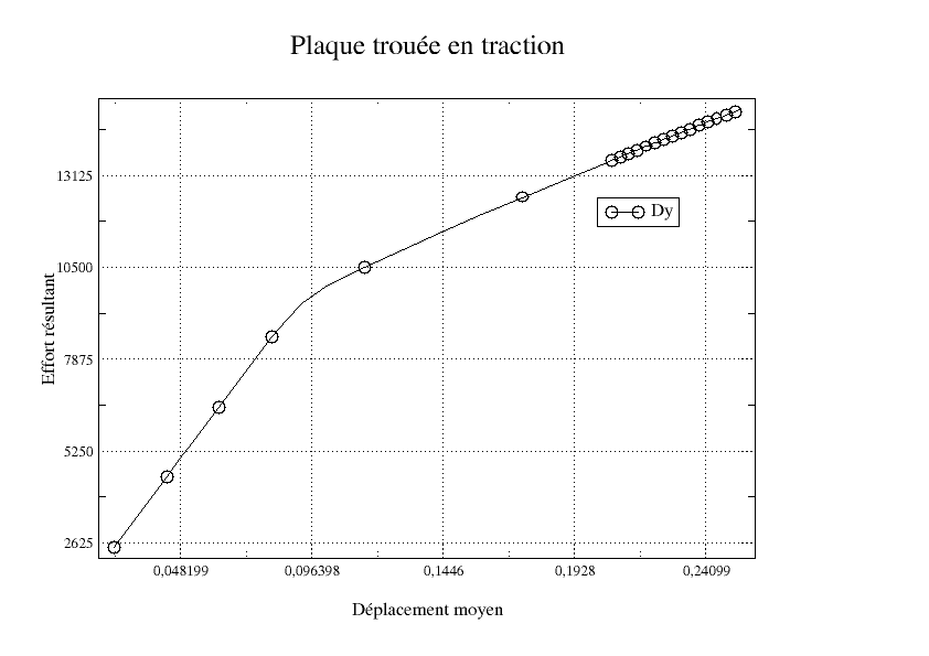
This example is extracted in part from test case [FORMA03a], it is a plate with holes in tension.
After a calculation carried out with STAT_NON_LINE, we want to plot the force resulting from traction as a function of the average vertical displacement of the upper part of the test piece.
Post-processing details:
POURSUITE ()
SOLNL2 = CALC_CHAMP (Calculation of nodal forces
reuse = SOLNL2, RESULTAT = SOLNL2,
OPTION = “FORC_NODA”,)
M= DEFI_GROUP (Definition of the group of nodes of
Reuse=m, stripping, the top line of the plate
MAILLAGE =M,
CREA_GROUP_NO =_F (GROUP_MA = “LFG”,
NOM = “LIGNE”,),
)
tab= POST_RELEVE_T (
ACTION =(
_F (INTITULE = “Umean”, Average travel record at all times
RESULTAT = SOLNL2, calculation times
NOM_CHAM = “DEPL”,
NOM_CMP = “DY”,
TOUT_ORDRE = “OUI”,
GROUP_NO = “LIGNE”,
OPERATION = “MOYENNE”,
),
_F (INTITULE = “Resultante”, Resultant effort statement
RESULTAT = SOLNL2,
NOM_CHAM = “FORC_NODA”,
TOUT_ORDRE = “OUI”,
GROUP_NO = “LIGNE”,
RESULTANTE = “DY”,
OPERATION = “EXTRACTION”,),),)
IMPR_TABLE (TABLE =tab,) Just to find the name of the parameters
Contents (partial, limited to the first 3 moments) of the table:
INTITULE NOEUD RESU NOM_CHAM NUME_ORDRE INST DY SIYY QUANTITE
Umedium - SOLNL2 DEPL 1 1.00000E+00 2.38745E-02 - MOMENT_0
Umedium - SOLNL2 DEPL 1 1.00000E+00 -3.70291E-04 - MOMENT_1
Umedium - SOLNL2 DEPL 1 1.00000E+00 2.36709E-02 - MINIMUM
Umean - SOLNL2 DEPL 1 1.00000E+00 2.40291E-02 - MAXIMUM
Umean - SOLNL2 DEPL 1 1.00000E+00 2.40597E-02 - MOYE_INT
Umean - SOLNL2 DEPL 1 1.00000E+00 2.36894E-02 - MOYE_EXT
Umedium - SOLNL2 DEPL 2 1.20000E+00 2.86494E-02 - MOMENT_0
Umedium - SOLNL2 DEPL 2 1.20000E+00 -4.44349E-04 - MOMENT_1
Umedium - SOLNL2 DEPL 2 1.20000E+00 2.84050E-02 - MINIMUM
Umedium - SOLNL2 DEPL 2 1.20000E+00 2.88350E-02 - MAXIMUM
Umedium - SOLNL2 DEPL 2 1.20000E+00 2.88716E-02 - MOYE_INT
Umedium - SOLNL2 DEPL 2 1.20000E+00 2.84273E-02 - MOYE_EXT
Umedium - SOLNL2 DEPL 3 1.40000E+00 3.34244E-02 - MOMENT_0
Umedium - SOLNL2 DEPL 3 1.40000E+00 -5.18504E-04 - MOMENT_1
Umedium - SOLNL2 DEPL 3 1.40000E+00 3.31393E-02 - MINIMUM
Umedium - SOLNL2 DEPL 3 1.40000E+00 3.36410E-02 - MAXIMUM
Umedium - SOLNL2 DEPL 3 1.40000E+00 3.36837E-02 - MOYE_INT
Umedium - SOLNL2 DEPL 3 1.40000E+00 3.31652E-02 - MOYE_EXT
[…]
Resulting - SOLNL2 FORC_NODA 1 1.00000E+00 2.50000E+03 - -
Resulting - SOLNL2 FORC_NODA 2 1.20000E+00 3.00000E+03 - -
Resulting - SOLNL2 FORC_NODA 3 1.40000E+00 3.50000E+03 - -
[…]
Dy= RECU_FONCTION (Filtering the table to extract \(\mathrm{Dy}=f(t)\)
TABLE = tab,
PARA_X = “INST”,
PARA_Y = “DY”,
FILTRE = (
_F (NOM_PARA = “INTITULE”,
VALE_K = “Medium”,),
_F (NOM_PARA = “QUANTITE”,
VALE_K = “MOMENT_0”,),),)
Fy= RECU_FONCTION (Filtering the table to extract \(\mathrm{Fy}=f(t)\)
TABLE = tab,
PARA_X = “INST”,
PARA_Y = “DY”,
FILTRE = (
_F (NOM_PARA = “INTITULE”,
VALE_K = “Result”,),),)
IMPR_FONCTION (Plot the ordinates of \(\mathrm{Fy}\) as a function of \(\mathrm{Dy}\)
UNITE = 29,
FORMAT = “XMGRACE”,
COURBE = (
_F (FONC_X = Dy,
FONC_Y = Fy,),),
TITRE = “Plate with holes in tract”,
LEGENDE_X = “Average displacement”,
LEGENDE_Y = “Resulting effort”,)
This gives us the following curve:
4.3. Drawing a large number of curves#
In some applications, it is necessary to draw numerous curves. Suppose we want to compare our results to 50 measurement points obtained elsewhere. It would then be tedious to define 50 files in astk and to use 50 different logical units in the command file!
All you have to do is use the « repe » type as a result in astk (cf. [U1.04.00]):

We then proceed as follows in the command file in PAR_LOT =” NON “in POURSUITE:
# definition of the 50 groups of counting nodes
lgrno = [:ref:` “point01”, “point02”, …, “point50” < “point01”, “point02”, …, “point50” >`]
# for each stripping node…
For point in lgrno:
unit = 29
# files DEPL_point0i .dat will be copied into Results/curbes/
DEFI_FICHIER (UNITE =unit, FICHIER =”. /REPE_OUT/DEPL_ “+point+”.dat”)
tab= POST_RELEVE_T (
ACTION =_F (INTITULE = “vonMises”,
RESULTAT = ResM,
NOM_CHAM = “SIEQ_ELNO”,
NOM_CMP = “VMIS”,
TOUT_ORDRE = “OUI”,
GROUP_NO = point,
OPERATION = “EXTRACTION”,),)
IMPR_TABLE (
UNITE = unit,
TABLE = tab,
FORMAT = “XMGRACE”,
NOM_PARA = (“INST”, “VMIS”),
# we « free » the unit to reuse it for the next curve
DEFI_FICHIER (UNITE =unit, ACTION =” LIBERER “)