2. Modeling fluid-elastic forces#
In Code_Aster, there are two different methods for modeling fluid-elastic forces that represent fluid-structure coupling efforts. The difference between the two methods is in relation to the nature and the complexity of the physical phenomena that the user wishes to consider and, consequently, the hypotheses taken when calculating the coupling forces.
The first method consists in calculating added matrices representing fluid-structure coupling with a potential approach. It is assumed that the structure only undergoes small deformations and that the fluid that surrounds it is perfect; the effect of shear in the fluid is then considered negligible. For the calculation of the added mass, the fluid is considered to be unsteady. As for the added stiffness and damping, these can only be calculated in the presence of a flow. In this case, we hypothesize that the flow is potential; we then neglect any effect related to the physics of rotational flow which may be important in configurations with detachment or at turbulent speeds.
The second method for modeling coupling efforts consists in determining the fluid-elastic transfer matrix, particular for a predefined configuration; a « configuration » being the whole: the structure and its geometry on one side and the flow and its properties on the other. The configurations that can be modeled with this method are:
Cross flow tube bundle
Stem under flow through an annular confinement (Control cluster)
Axial flow tube bundle
Flow between two coaxial shells
Despite its sometimes restrictive hypotheses, the potential method nevertheless remains the most generic in terms of its applicability independent of the configuration of the study. The user is advised to use the second method only if his case study corresponds to one of the four configurations currently available.
2.1. The « potential » approach for calculating the modal base of a coupled system#
In this approach, the calculation method consists in determining, first of all, added mass, stiffness, and fluid damping matrices using the operator CALC_MATR_AJOU or the macro command MACRO_MATR_AJOU. These two operators result in added matrices, projected on the modal basis of the structure in a vacuum.
To determine the modal basis of the « wet » structure, simply combine the structural matrices with the generalized added matrices using the COMB_MATR_ASSE operator. Then you will have to do the natural mode calculation again by CALC_MODES. The modes of the coupled system must finally be restored on the physical basis of the structure with the help of operator REST_GENE_PHYS. The calculation steps are detailed in the following diagram:
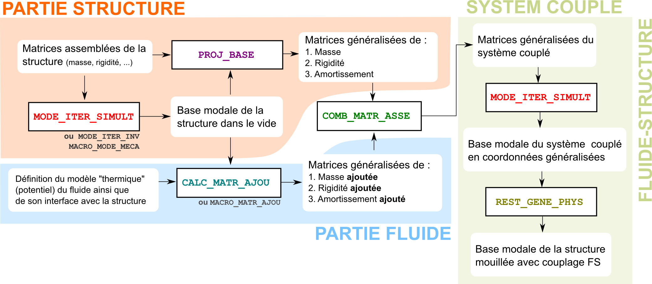
Figure 2.1-a : Scheme for calculating the modal base of a structure wetted by the potential approach
2.2. The « predefined configuration » approach for calculating the modal base of a coupled system#
The data entry and calculation method for this second approach is different from that in the potential approach. In fact, the physical phenomena that are modelled here are more complex and the results depend on an additional parameter, the speed of the flow. The calculation of a modal base of the coupled system is therefore established for a range of speeds. With this approach, we therefore obtain not a traditional dynamic modal base (mode_meca), but a fluid-elastic modal base, which will be called melasflu in Code_Aster.
To calculate the fluid-elastic base of a coupled system, the user must first call operator DEFI_FLUI_STRU to fill in the type of configuration of his study as well as all the characteristics associated with it. These characteristics differ according to the configuration but they generally concern the geometry of the structure, the properties of the fluid and its flow.
2.2.1. Special case of a bundle of tubes under transverse flow#
In the case of the configuration of a bundle of tubes under transverse flow (FAISCEAU_TRANS), it is possible to calculate by means of the operator FONC_FLUI_STRU, the inertial distribution of the fluid throughout the structure. The user can therefore use this information to enrich the structural matrices before carrying out his first modal calculation of the structure. In practice, after the call to FONC_FLUI_STRU, the user must create a fluid-structure hybrid material using the ELAS_FLUI option of DEFI_MATERIAU and assign it to all elements of the structure under transverse flow (AFFE_MATERIAU).
The elementary mass and stiffness matrices can then be calculated with the options MASS_FLUI_STRU and RIGI_FLUI_STRU of CALC_MATR_ELEM. After assembling the elementary matrices, the user will be able to calculate the modal base of the wet structure, for example with the operator CALC_MODES.
It is important to note that this consideration, beforehand, of the inertial effect of the fluid is only possible in the case of a bundle of tubes under transverse flow. It makes it possible to subsequently perform all of the dynamic analysis on a projection basis that corresponds to the modal basis of the wet structure.
2.2.2. Case of other configurations#
For the other three configurations, the modal reference base is determined on the basis of the mechanical properties of the structure (purely structural mass and stiffness matrices), without taking into account at this level the effects associated with the presence of the fluid.
Once the configuration of the study and the reference projection base are well defined, the study of the coupled system can continue with a call to operator CALC_FLUI_STRU. This operator retrieves, in addition to the configuration of the study and the projection base, a list of velocities that represent the range of flow velocities over which the user wishes to study the dynamic behavior of its structure.
In the concept resulting from CALC_FLUI_STRU, the user has for each flow speed, a base modified by taking into account all the fluid-elastic coupling coefficients. The calculation steps for the four configurations are detailed in the following two diagrams:
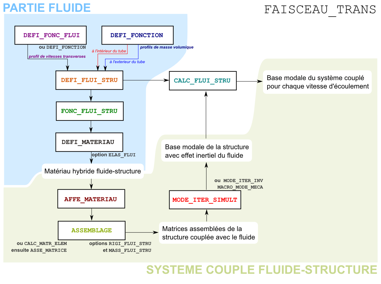
Figure 2.2.2-a : Scheme for calculating the modal base of a bundle of tubes under cross flow
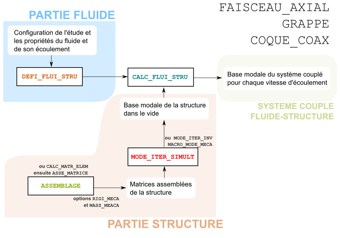
Figure 2.2.2-b : Scheme for calculating the modal base of structures in one of the 3 configurations: bundle of tubes under axial flow, control cluster, and flow between 2 coaxial shells.
2.3. Vibratory analyses following the obtaining of the modal base of the coupled system#
The modeling of fluid-elastic forces is almost complete with the obtaining of a dynamic modal base of the structure taking into account the effects of coupling. To continue his study, the user can freely use the calculated modal base to analyze the behavior of his fluid-structure coupled system.
Transient analysis
In the case where the modeling of the fluid-elastic coupling was carried out according to the second method, that is to say on the basis of a predefined configuration in the operator DEFI_FLUI_STRU, the user must use the operator MODI_BASE_MODALE in order to extract from the melasflu base, a modal base of the mode_meca type for a single flow speed. The modal base will then be usable in all transient dynamics operators.
In the case where added coefficients have been calculated according to the potential method, the user can directly use the modal base obtained by restoring the generalized modes base on a physical basis (result of the call to REST_GENE_PHYS, see).
There is currently only one temporal integration scheme that accepts modal bases of type melasflu , it is the ITMI method of the operator DYNA_VIBRA .
Spectral analysis
However, to perform a dynamic spectral analysis of the coupled system, the user is not required to extract a mode_meca database from its wet melasflu base. The operator DYNA_SPEC_MODAL, which allows spectral analyses to be carried out, is in fact compatible with modal bases such as melasflu.