6. Code_Aster test case#
To implement the calculation of complex modes on a reduced model, a simple example is introduced. The calculation of the modes on this structure will be carried out with*Code_Aster.* The results obtained will be compared using the complete model first, then various reduced models. The typical command file used to perform this calculation will then be detailed, with emphasis on points not covered in the official documentation.
6.1. Note on the studies presented#
The command files used for the calculations of the complex modes of the reduced models are available in the studies database, under the study number 3185. They do not present an optimized way of carrying out calculations, in particular in the calculation of residues and the construction of projection bases. On this point, it should be noted that developments have been studied to optimize this procedure.
However, it is a question of illustrating the approach to allow the user to reproduce and adapt the methodology.
The main points of interest are highlighted. It is mainly about:
The definition of materials: In fact, materials must be defined « doubly » to calculate residues
It is necessary to assign hysteretic damping to each material, otherwise it will not be properly taken into account. For non-dissipative materials, it is therefore necessary to set zero hysteretic damping.
The options for the eigenmode solver: The latter must be used with the « CENTRE » option only, even if the modes you are looking for are the first in the structure The other options are not supported by the solver.
6.2. Numerical example with hysteretic damping#
The example used for this study is a square plate with a side of 1 meter and 6 centimeters thick, composed of a sandwich material steel/viscoelastic material/steel. The layers are linear, elastic and isotropic, perfectly glued and 2 centimeters thick. The finite element model is shown on Figure 6.2-a. This plate is embedded on one edge, and we are interested in the first 10 modes of this structure. The Young’s modulus of the viscoelastic material is not realistic. It has been adjusted to obtain reasonable amortization, despite the thickness of the layer. These properties are recalled in Tableau 6.2-1.
Material |
Young’s Modulus (\(\mathit{Pa}\)) |
Poisson’s Ratio |
Density (\({\mathit{kg.m}}^{\mathrm{-}3}\)) |
Rate of loss |
Steel |
2.1.1011 |
0.3 |
7800 |
0.0 |
Visco |
1.5.1010 |
0.49 |
1400 |
1.0 |
Table 6.2-1: Properties of the materials used for the calculation.
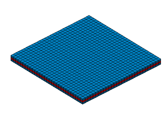
Figure 6.2-a: E.F. model of the reference structure.
The model is built using linear solid elements, with a total of 9610 nodes, or 27900 degrees of freedom.
The first 10 modes of the damped structure are calculated using Code_Aster. In each case, the calculation is carried out on a reduced model built from the first 20 normal modes only (base \({T}_{20}\)), and a reduced model built from the first 10 normal modes enriched with the residues associated with these 10 normal modes (base \({T}_{10+10}\)). A reference calculation carried out with the complete non-reduced model is also carried out. The reduction bases used are therefore
and
The results obtained with the various models are presented in Tableau 6.2-2 and Tableau 6.2-3.
Complete |
Base \({T}_{20}\) |
Base \({T}_{10+10}\) |
Full Relative Error/Modes (%) |
Full Relative Error/Residue (%) |
|
61.84 |
61.39 |
61.39 |
61.84 |
-0.73 |
0 |
138.71 |
135.24 |
138.7 |
-2.5 |
-0.01 |
|
357,37 |
345,84 |
357,84 |
357,36 |
-3,23 |
0 |
449.34 |
436.52 |
449.29 |
449.29 |
-2.85 |
-0.01 |
485.45 |
465.42 |
485.42 |
485.41 |
-4,13 |
-0.01 |
533.39 |
533.27 |
533.4 |
-0.02 |
0 |
|
803.6 |
764.05 |
803.49 |
-4.92 |
-0.01 |
|
935.99 |
886.65 |
935.65 |
935.76 |
-5.27 |
-0.02 |
998.4 |
949.07 |
998.24 |
-4.94 |
-0.02 |
|
1053.3 |
995.94 |
1053.2 |
-5.45 |
-0.01 |
-0.01 |
Table 6.2-2: Natural frequencies (in Hz) of the sandwich model.
The frequencies calculated from the reduced model on 10 modes and 10 residues are almost identical to those calculated using the complete model. The frequencies obtained from the reduced model based on the first 20 normal modes are reasonable, but nevertheless present a significant error.
Complete |
Base \({T}_{20}\) |
Base \({T}_{10+10}\) |
Full/Modes |
Full/Residues |
|
1.4 |
2.16 |
1.4 |
54.29 |
0 |
|
3.78 |
6.07 |
3.74 |
3.74 |
60.58 |
-1.06 |
4.95 |
8.07 |
4.93 |
4.93 |
63.03 |
-0.4 |
4.3 |
6.9 |
4.27 |
4.27 |
60.47 |
-0.7 |
6.55 |
10.28 |
6.51 |
56.95 |
-0.61 |
|
1.91 |
1.91 |
1.9 |
1.9 |
0 |
-0.52 |
8.33 |
12.71 |
8.27 |
52.58 |
-0.72 |
|
9.3 |
13.9 |
9.29 |
9.29 |
49.46 |
-0.11 |
8.08 |
12.55 |
8.06 |
55.32 |
-0.25 |
|
9.35 |
14.12 |
9.21 |
9.21 |
51.02 |
-1.5 |
Table 6.2-3 : Depreciation (in%) of the sandwich model.
On the other hand, the calculation of reduced depreciation is much more precise. The results obtained with the reduced model on normal modes only, with the exception of mode 6, lead to a very clear overestimation of damping. Integrating residuals into the model’s reduction base greatly improves the results. The maximum error in the calculation, compared to the reference model, is in fact just greater than one percent, for a projection base of equivalent size in both cases.
6.3. Numerical example with viscoelastic damping described by internal variables#
The same geometry was used to build this study. However, it is not possible to build reference test cases, using the non-reduced model, with*Code_Aster*. The reference results, calculated on the complete model, were therefore obtained with Matlab and the*Structural Dynamic Toolbox*. The characteristics of the materials used are shown in the table.
Material |
Young’s module (\(\mathit{Pa}\)) |
Poisson’s ratio |
Density (\({\mathit{kg.m}}^{\mathrm{-}3}\)) |
Relaxation time (\(s\)) |
Steel |
2,1.1011 |
0.3 |
7800 |
\(\infty\) |
Visco |
4,53.106 |
0.49 |
1400 |
\(\infty\) |
3,51.106 |
0.49 |
5,58.10-2 |
||
1,395.107 |
0.49 |
3,20.10-3 |
||
4,04.107 |
0.49 |
3,01.10-4 |
||
1,20.108 |
0.49 |
4,58.10-5 |
||
7,57.108 |
0.49 |
5,93.10-6 |
Table 6.3-1 : Properties of the materials used.
The results obtained with the full model and the reduced model are shown in the table. The scale model was built on the basis of the first ten natural modes of the non-dissipative structure.
Complete |
Reduced |
||
Freq. (\(\mathit{Hz}\)) |
Love. (%) |
Freq. (\(\mathit{Hz}\)) |
Love. (%) |
25,26 |
7.00 |
25,26 |
7.00 |
48.41 |
10.60 |
47.96 |
10.85 |
150.61 |
8.55 |
150.59 |
8.55 |
174.11 |
11.39 |
174,07 |
11.40 |
186,38 |
8,69 |
186.17 |
8.88 |
309,68 |
10,10 |
309,64 |
10,11 |
426.46 |
8.04 |
426.36 |
8,08 |
438,48 |
9.80 |
439.97 |
10.31 |
463,72 |
8,93 |
463.77 |
8,98 |
523.22 |
0.04 |
523.22 |
0.04 |
Table 6.3-2 : Comparison of results — Frequencies and damping.
The results obtained are very good, and the error for the first ten modes is very low, both in terms of frequencies and damping.