4. Recommendations for use#
4.1. Introduction of the theta field#
4.1.1. Conditions to be respected#
Field \(\theta\) is a vector field, defined on the cracked solid, which represents the transformation of the domain during crack propagation. This field should meet the following conditions:
the transformation should only change the position of the crack bottom and not the edge of the \(\partial \Omega\) domain. Field \(\theta\) must therefore be tangent to \(\partial \Omega\) (in particular the lips of the crack), i.e. by noting \(n\) the normal to \(\partial \Omega\): \(\theta \mathrm{.}n=0\mathrm{sur}\partial \Omega\).
Field \(\theta\) must be locally in the tangential plane to the lips of the crack and in 3D normal to the edge to which it belongs. This corresponds to the direction of propagation of the crack.
Field \(\theta\) must also be continuous on \(\Omega\).
4.1.2. Advice on choosing Rinf and Rsup crowns#
In Code_Aster, the choice was made to define field \(\theta\) as follows:
the direction of the field is collinear to the direction of propagation of the crack. In 3D, we take the local direction of the projection of the node in question on the crack background;
the \(\theta\) standard is defined using two crowns (or tori in 3D), with radii \({R}_{\text{inf}}\) and \({R}_{\text{sup}}\). Below \({R}_{\text{inf}}\), the module of the theta field is constant and equal to 1, beyond that it is zero and it is linear between the two, cf.

Figure 4.1.2-1 : Geometric definition of the theta field
The construction of the theta field is described precisely in [R7.02.01]. It is implemented in command CALC_G.
In 2D and axisymmetric, the bottom of crack \({\Gamma }_{0}\) is limited to one point. The user defines:
rays \({R}_{\text{inf}}\) and \({R}_{\text{sup}}\),
In 3D the user defines:
rays \({R}_{\text{inf}}(s)\) and \({R}_{\text{sup}}(s)\),
the topology of the crack bottom: open or closed depending on whether the crack is open or not,
Note:
The displacement and stress fields are singular at the bottom of the crack; the precision of the calculation is therefore lower in the vicinity of the bottom. Note that the shape of the theta field chosen ( \(\theta \mathrm{.}m\) constant between 0 and \({R}_{\text{inf}}\) ) precisely makes it possible to cancel the contribution of the classical term of \(G(\theta )\) inside the first ring (term en \({\int }_{\Omega }\left[\sigma (u):(\nabla u\mathrm{.}\nabla \theta )-\Psi (\varepsilon (u))\text{div}\theta \right]d\Omega\) ) .
Do not forget that loads applied beyon \({R}_{\text{sup}}\) have a zero contribution in fracture mechanics post-treatments. This can be useful if you apply a loading that is not supported like FORCE_NODALE, DDL_IMPO (in 2D) or FACE_IMPO (in 3D) .
Advice on the choice of radius \({R}_{\text{inf}}\) and \({R}_{\text{sup}}\) : the calculation of fracture mechanics quantities is theoretically independent of the choice of the integration ring (in the absence of loading on the lips, volume or thermal). However, it is best to respect a few rules:
never take \({R}_{\text{inf}}\) or too small in relation to the dimensions of the problem because the singular displacements are poorly calculated in the vicinity of the crack bottom (see note above);
the upper radius \({R}_{\text{sup}}\) can be as big as you want provided that the corona thus defined is contained in the solid. In 3D, you should not take a \({R}_{\text{sup}}\) radius that is too large, otherwise the direction of the theta field (calculated by projection onto the crack background) may be inaccurate;
the choice of radii \({R}_{\text{inf}}\) and \({R}_{\text{sup}}\) is independent of the topology of the mesh. However, if the mesh is radiant at the crack point, it is recommended to take integration rings that are coincident with the mesh crowns (reduction of oscillations by \(G\) along the crack bottom in 3D);
In thermo-elastoplasticity, a crack is used as a cut. Make sure that the lower radius \({R}_{\text{inf}}\) is much greater than the radius of the notch.
Take several consecutive crowns to check [R1,R2], [R2,R3], [R3, R4],…
To get started, for a crack of length a in an infinite medium, the size of the elements at the bottom of the crack must be less than \(a/10\) to obtain a reasonable error (of the order of% on \(\mathrm{K1}\)). For integration rings, we then generally take \({R}_{\text{inf}}\) of the order of 1 to 3 times the size of the elements in the vicinity of the background; and \({R}_{\text{sup}}\) of 3 to 7 times the size of the elements.
An automatic determination of \({R}_{\text{inf}}\) and \({R}_{\text{sup}}\) is possible (these keywords are optional). If they are not specified, they are automatically calculated from the maximum \(h\) of the mesh sizes connected to the nodes at the bottom of the crack. It was chosen to take \({R}_{\text{sup}}\mathrm{=}4h\) and \({R}_{\text{inf}}\mathrm{=}2h\). If you choose the value automatically calculated for \({R}_{\text{inf}}\) and \({R}_{\text{sup}}\), you must however ensure that these values (displayed in the .mess file) are consistent with the dimensions of the structure.
4.1.3. Discretization problem in 3D#
In 3D, for a current node at the crack bottom, the direction of propagation is defined as being the average of the normals to the mesh segments of the crack bottom to its left and to its right. For end nodes, the normal is calculated from a single mesh, and may therefore be less accurate or even false.
Fissure emerging orthogonally to the edges: the propagation direction vectors at the origin and at the end of the bottom are automatically calculated taking into account the edges of the structure. The keywords DTAN_ORIG and DTAN_EXTR (command DEFI_FOND_FISS for calculating G on a mesh crack), which make it possible to impose the direction of these vectors, therefore do not need to be specified.
Crack emerging in a non-perpendicular way: at the through end of the crack bottom, field \(\theta\) cannot simultaneously be normal to the edge to which it belongs (in the tangential plane of the crack lips) and verify condition \(\theta \mathrm{.}n=0\) on \(\partial \Omega\).
The recommended solution is to impose as the direction of propagation at the ends (keywords DTAN_ORIG and DTAN_EXTR) the average of the normal at the bottom of the crack at this point \({\theta }_{1}\) and of the tangent to the edge \({\theta }_{2}\).

Figure 4.1.3-1: Direction of propagation at the ends of the crack
4.2. 3D interpolation methods#
4.2.1. General framework#
The local energy recovery rate \(G(s)\) is a solution to the variational equation \({\int }_{{\Gamma }_{0}}G(s)\theta (s)\mathrm{.}m(s)\mathrm{ds}=G(\theta ),\forall \theta \in \Theta\).
To solve this equation:
we decompose the scalar field \(G(s)\) on a basis that we denote \({({p}_{j}(s))}_{1\le j\le N}\). Let \({G}_{j}\) be the components of \(G(s)\) in this base: \(G(s)=\underset{j=1}{\overset{N}{\Sigma }}{G}_{j}{p}_{j}(s)\).
We give ourselves a base of test functions for \(\theta\) by choosing \(P\) fields \({\theta }^{i}\) independent for the trace of field \(\theta\) on the crack background \({\Gamma }_{0}\): \({(\stackrel{ˉ}{{\theta }^{i}}(s))}_{1\le i\le P}\).
The \({G}_{j}\) are determined by solving the linear system at

equations and

unknowns:
\(\underset{j=1}{\overset{N}{\Sigma }}{a}_{\mathrm{ij}}{G}_{j}={b}_{i},i=\mathrm{1,}P\)
with \(\begin{array}{}{a}_{\mathrm{ij}}=\underset{k=1}{\overset{M}{\Sigma }}{\theta }_{k}^{i}{\int }_{{\Gamma }_{O}}{p}_{j}(s){q}_{k}(s)\mathrm{.}m(s)\mathrm{ds}\\ {b}_{i}=G({\theta }^{i})\end{array}\)
This system has a solution if we choose \(P\) independent \({\theta }^{i}\) fields such as:

What if

. It may have more equations than unknowns, in which case it is solved in a least-squares sense.
4.2.2. G and Theta smoothing methods#
In Code_Aster, two families of bases were chosen (cf. [§2.2]):
the polynomials of LEGENDRE \({\gamma }_{j}(s)\) of degree \(j\) (\(0=j=7\)),
the shape functions of node \(k\) from \({\Gamma }_{0}\):

(\(\mathrm{1 }=k=\mathrm{NNO}\) = number of \({\Gamma }_{0}\) nodes) (degree1 for linear elements and degree2 for quadratic elements).
These families of bases and the linear systems to be solved are precisely described in the reference documentation [R7.02.01]. The use of form functions is called “LAGRANGE” in Code_Aster, a variant of which is available:
“LAGRANGE_NO_NO”: simplified version of smoothing LAGRANGE, allowing in some cases to obtain more regular results at the bottom of a crack.
Several options are therefore possible depending on the test function base for theta and the decomposition base for \(G\). They are summarised in the following table:
Theat |
|||
Polynomials of LEGENDRE |
Shape features |
||
\(G(s)\) |
Polynomials of LEGENDRE |
LISSAGE_THETA = “LEGENDRE” LISSAGE_G = “LEGENDRE” |
LISSAGE_THETA =” LAGRANGE “LISSAGE_G =” LEGENDRE “ |
Shape features |
LISSAGE_THETA = “LAGRANGE” LISSAGE_G = “LAGRANGE” or “LAGRANGE_NO_NO” |
||
Table 4.2.2-1: Possible combinations for calculating \(G\) in 3D
4.2.3. Notes and tips#
Choice of method: it is difficult to give preference to one or the other method. In principle, both give equivalent numerical results. However, the Theta: Lagrange method is a bit more expensive in time CPU than the Theta: Legendre method. It is essential to use several methods and to compare results, in order to confirm the validity of the model.
Choice of the maximum degree of Legendre polynomials: this choice depends on the number of nodes at the bottom of the crack. If you have a low number of nodes (about ten) it is useless to take a degree greater than 3 (you can easily imagine that the results are poor if you try to find a polynomial of degree 7 passing through 10 points). Beyond twenty knots at the bottom of a crack, degrees of up to 7 can be used. Experience shows that choosing a degree equal to 5 gives good results in most cases (see note below).
Case of closed cracks: if the crack bottom is a closed curve, problems of continuity of the solution at the point arbitrarily chosen as the origin curvilinear abscissa prevent the use of Legendre polynomials. If the crack bottom was declared « closed » in DEFI_FOND_FISS, you should use the shape functions (Lagrange) to describe the functions \(G\) and \(\theta\).
Problem of not respecting symmetry: if we only model half of the solid with respect to the crack, we should in principle have a \(G(s)\) curve whose tangent slope is zero at the symmetry interface. This is not respected by both methods. Values of \(G(s)\) obtained at the ends of the crack bottom should always be interpreted with caution, especially if the crack opens in a non-perpendicular manner (see § 4.1.3).
Oscillation problem with Lagrange: oscillations may occur with the Lagrange method, especially if the mesh includes quadratic elements. These oscillations are linked to a radial profile of the theta field that is different on the vertex nodes and on the middle nodes. A smoothing of the “LAGRANGE_NO_NO” type makes it possible to limit these oscillations. Moreover, if the mesh is radiating at the bottom of the crack (mesh crack), it should be noted that it is recommended to define crowns R_ INFet R_ SUPcoïncidant with the borders of the elements.
Case of free meshes: strong oscillations may occur with the Lagrange method. Smoothing like “LAGRANGE_NO_NO” limits these oscillations, but may not be sufficient. In this case, it is recommended to use the NB_POINT_FOND operand from CALC_G. The choice of a ratio of the order of 5 between the total number of points at the bottom of the crack and the number of calculation points seems appropriate to limit oscillations with the Theta: Lagrange method. A choice of 20 points at the bottom of a crack is often wise.
Performance: the NB_POINT_FOND operand can also be used to reduce the calculation time of CALC_G.
Illustration of oscillation problems with Legendre: is a case where the solution is constant on the background of crack \({G}^{\mathrm{exact}}(s)={\gamma }_{0}(s)\). If the term in front of the Legendre polynomial of degree seven is miscalculated, within a factor of \(\varepsilon\) (but all the other coefficients in front of the other polynomials are exactly 0), then the numerical result is: \(G(s)={\gamma }_{0}(s)+\varepsilon \cdot {\gamma }_{7}(s)\). So the relative error made on \(G\) is:
\(e=\frac{G(s)-{G}^{\mathrm{exact}}(s)}{{G}^{\mathrm{exact}}(s)}=\varepsilon \cdot \frac{{\gamma }_{7}(s)}{{\gamma }_{0}(s)}=\varepsilon \sqrt{15}\frac{{P}_{7}(\frac{\mathrm{2s}}{l}-1)}{{P}_{0}(\frac{\mathrm{2s}}{l}-1)}=\varepsilon \sqrt{15}{P}_{7}(\frac{\mathrm{2s}}{l}-1)\).
If we plot the \(\frac{e}{\varepsilon }\) ratio as a function of the normalized curvilinear abscissa \(\frac{s}{l}\), we get the following figure.
The error at the ends (in \(x=0\) and \(x=\frac{s}{l}\)) is about 2 to 3 times greater than the maximum error at the bottom. For example, if \(\varepsilon\) is equal to \({10}^{-2}\) (i.e. 1% error), we will commit a maximum error of 1.5% everywhere, except at the extremes where the error will reach 4%.
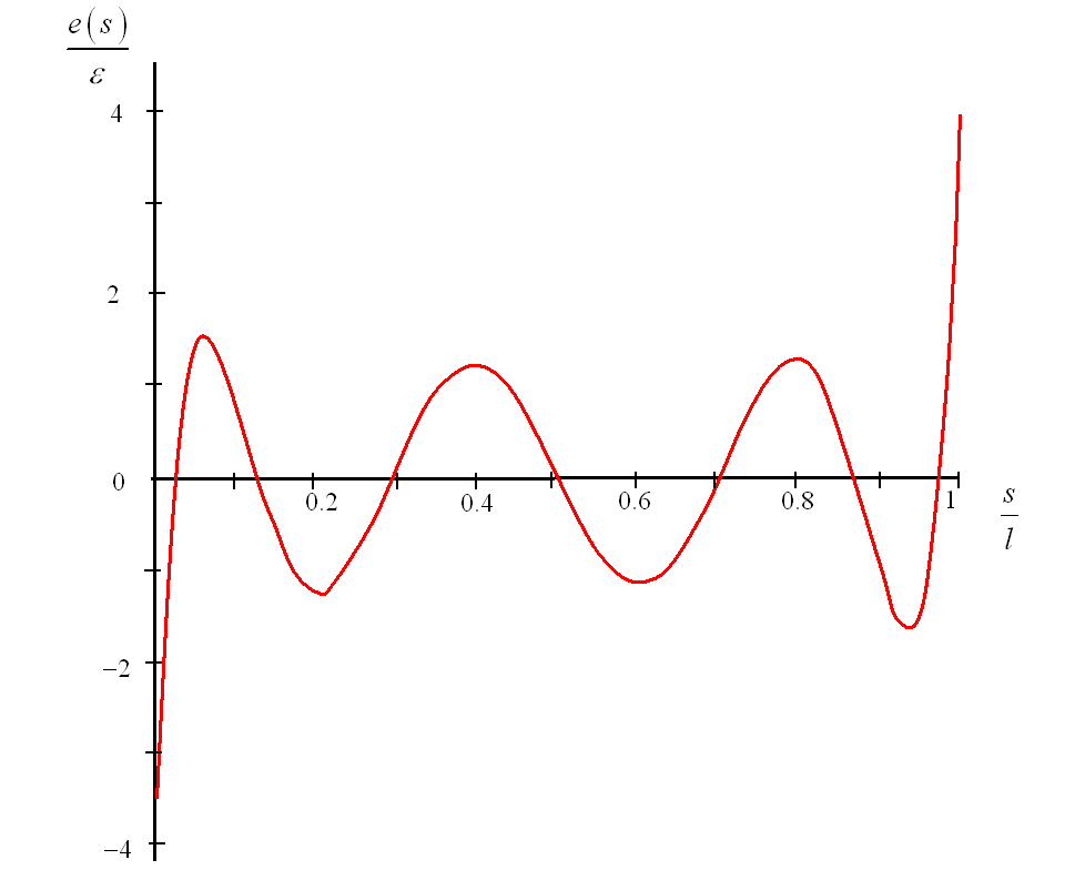
Figure 4.2.3-1: Relative error to precision ratio as a function of the standard curvilinear abscissa
4.3. Tips for calculations with POST_K1_K2_K3#
Choice of extrapolation distance: Extrapolation distance ABSC_CURV_MAXI is the only user parameter. In general, this distance is chosen to be equal to 3 to 5 times the size of the elements in the vicinity of the crack bottom. In the case of a mesh crack, the ABSC_CURV_MAXI parameter is optional. The default value is then equal to \(4h\) where \(h\) is the maximum size of the cells connected to the nodes at the bottom of the crack.
Case of mesh cracks: the mesh must preferably be quadratic and have enough nodes perpendicular to the crack bottom. On the other hand, the results are significantly improved if, in the case where the mesh is composed of quadratic elements, the middle nodes (edges that touch the bottom of the crack) are moved to a quarter of these edges by bringing them closer to the bottom of the crack. This is made possible by the MODI_MAILLE keyword (option “NOEUD_QUART”) in the MODI_MAILLAGE [U4.23.04] command.
Case of non-meshed cracks: the precision of the method is sensitive to the choice of the enrichment zone for the X- FEM method (parameter RAYON_ENRI of DEFI_FISS_XFEM). Ideally, the radius of enrichment and the maximum curvilinear abscissa ABSC_CURV_MAXI are of the order of three times the size of the minimum edge of the mesh.
Performance: in the case of X- FEM, the calculations are quite time-consuming and memory-intensive if there are a lot of points on the bottom of the crack. The use of the NB_POINT_FOND keyword makes it possible to limit post-processing to a certain number of points evenly distributed along the background.
4.4. Normalization, symmetries#
4.4.1. 2D plane stresses and plane deformations#
In dimension 2 (plane stresses and plane deformations), the crack bottom is reduced to one point and the value \(G(\theta )\) from the CALC_G command is independent of the choice of field \(\theta\):
\(G=G(\theta )\forall \theta \in \Theta\)
4.4.2. Axisymmetry#
In axisymmetry it is necessary to normalize the value \(G(\theta )\) obtained with Code_Aster for the options CALC_G, G_ MAX and G_ BILI:
\(G=\frac{1}{R}G(\theta )\)
where*R* is the distance from the crack bottom to the axis of symmetry [R7.02.01 §2.4.4].
For option CALC_K_G, the values of \(G\) and \(K\) provided in the result table are directly the local values, so they should not be normalized.
4.4.3. 3D#
In dimension 3, the value of \(G(\theta )\) for a given \(\theta\) field is such that:
\(g(\theta )={\int }_{{\Gamma }_{0}}G(s)\theta (s)\mathrm{.}m(s)\mathrm{ds}\)
By default, the direction of field \(\theta\) at the bottom of the crack is normal to the bottom of the crack in the plane of the lips. By choosing a unit \(\theta\) field in the vicinity of the crack bottom, we then have:
\(\theta (s)\mathrm{.}m(s)=1\)
and:
\(G(\theta )={\int }_{{\Gamma }_{0}}G(s)\mathrm{ds}\)
4.4.4. Model symmetry#
It is possible to take into account a possible symmetry of the problem treated directly on the calculation of the \(G\) energy return rate and the stress intensity factors. See the SYME keyword in CALC_G [U4.82.03] and POST_K1_K2_K3 [U4.82.05].