5. Quality control of calculated solutions#
5.1. Quantities of interest from the quasistatic#
As with quasistatic calculations, we can classify the quantities relevant for post-treatment into two categories [bib1]:
evolutions such as force/displacement: quantities making it possible to interpret the overall response of the structure,
field isovalues such as damage or cumulative plastic deformation.
5.2. Additional dynamic quantities to be analyzed#
In addition to these analyses, for dynamic calculations, it is essential to verify that the hypothesis of slow evolution is respected. To do this, it is necessary to ensure that the inertial forces remain weak compared to the other forces in the system (external and internal forces). A simple way to have an evaluation of the evolution of inertia forces during the calculation consists in observing the acceleration field over time.
A first simple criterion can be based on a (infinite) norm of acceleration at each moment. In the event of a significant and lasting increase in acceleration (for example beyond 1 m/s2 over several consecutive time steps), this means that dynamic phenomena (therefore not taken into account by a quasi-static resolution) occur:
if we are in a physical framework, therefore with a realistic density, the calculated solution is therefore subject to significant dynamic phenomena;
if we are in an explicit framework where the density has been multiplied to increase the critical time step, then the inertia effects observed are a sign that the resolution method is not suitable. It is then imperative to modify the parameters, such as lowering the density, modifying the damping, etc.
In the first case, we can try to restart a calculation with a slightly finer step and possibly a slightly higher Rayleigh damping, or even with a typical HHT scheme. If, even with all these modifications, the solution still has inertia effects, then any quasistatic approach is unsuitable.
5.3. Analysis examples#
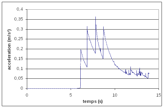
On the graph below (small reinforced concrete structure), we present a case where the acceleration will become significant, starting at 6 s. The maximum value remains less than 0.4 m/s2 and we are in a case with realistic density. Moreover, the acceleration will become weak again after 10 s: from all this we can conclude that the calculation remains compatible with the hypothesis of slow evolution.
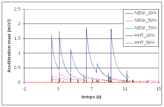
On the following graph, we can quantify the influence of damping (due to Rayleigh and the diagram) on maximum acceleration. Overall, in this example, the use of a HHT schema with Rayleigh damping set to an equivalent modal value of 20% is well suited (black curve). On the other hand, the mean acceleration scheme (Newmark) will only allow acceleration to be controlled if it is coupled with very significant Rayleigh damping: 50% equivalent modal damping. The calculated solution then risks being too dissipative.
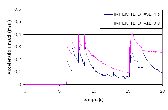
In the following figure, we can judge the influence of a discretization parameter: the time step, in terms of controlling the maximum acceleration. The value of 10-3 s for the time step is not well chosen and it is therefore preferable to divide the time step by two. To analyze this behavior, it is essential to conduct a parametric study on the time step.
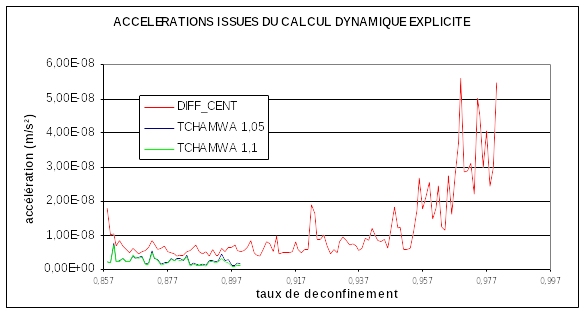
In the case of an explicit resolution (on an example very different from the previous ones: excavation of a circular gallery [bib1]) we compare different time schemes: the centered differences (therefore without induced damping) and the Tchamwa diagram for two values of the parameter PHI. The larger this parameter, the more high-frequency damping is introduced and this damping becomes zero for PHI =1.
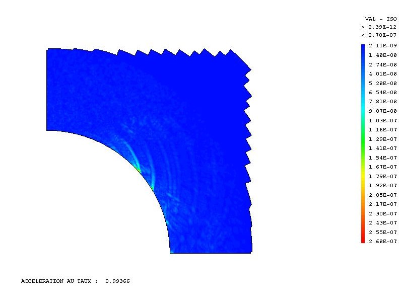
In addition to the previous curves, it is instructive to visualize some isovalues of the acceleration norm (for the same example of explicit excavation):
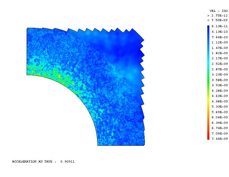
In the figure on the left, we are in a phase of low acceleration (the non-linearity associated with the deconfinement rate is still low). The shape of the acceleration field is quite random: one cannot perceive a « pattern » betraying a real dynamic phenomenon.
In the figure on the right, non-linearity is established and a very different acceleration distribution is observed: we can see the appearance of shear bands around the perimeter of the excavation. But even in this case, the maximum acceleration values remain very low (including taking into account the density increase factor). The solution obtained explicitly is therefore relevant in the sense of slow evolution.