8. Bibliography

[1] D. BERNAUD and G. ROUSSET: The « new implicit method » for the study of the sizing of tunnels, Revue Française de Géotechnique no. 60, pp 5-26, - 1992

[2] P. CATEL: Aval du Cycle — Bure site — Site de Bure — Sheet 13 — Convergence-confinement method, note EDF TEGG EFT GG/00 168 A — 2000

[3] A. GIRAUD: Thermo-Hydro-Mechanical Couplings in poorly permeable porous media: application to deep clays, thesis from ENPC — 1993

[4] D. LE BOULCH: Comparison of the THM 3D and 2D models of a storage structure with the Code_Aster, report Ajilon Technologies CÉnergys 01-A — 2002

[5] M. PANET: The calculation of tunnels by the convergence-confinement method, Presses de l’ENPC — 1995

[6] N. SELLALI, C. CHAVANT and G. DEBRUYNE: Hydroplastic modeling of the excavation of an underground gallery with the Code_Aster, note EDF MMN HI-74/00/009/A — 2000

[7] N. SELLALI, C. CHAVANT and G. DEBRUYNE: THM modeling of an underground storage structure with the Code_Aster, note EDF MMN HI-74/01/014/A — 2001

Analytical formulas to apply the convergence-confinement method in the case of an elastic and linear rock mass and support

The medium is assumed to be isotropic linear elastic and subject to an initial stress field that is also isotropic (\({K}_{0}\mathrm{=}1\)).

Radial stress, orthoradial stress and radial displacement at the tunnel wall in an elastic medium subject to a deconfinement rate \(\mathrm{\lambda }\)

\(\{\begin{array}{}{\sigma }_{R}=(1-\frac{\lambda \text{.}{R}^{2}}{{r}^{2}})\text{.}{\sigma }^{0}\\ {\sigma }_{\mathrm{\theta }}=(1+\frac{\lambda \text{.}{R}^{2}}{{r}^{2}})\text{.}{\sigma }^{0}\\ {U}_{R}=\lambda \cdot \frac{{R}^{2}}{r}\cdot \frac{{\sigma }^{0}}{\mathrm{2G}}\end{array}\)

\(G\) is given by the following relationship: \(G=\frac{E}{2\cdot (1+\mathrm{\nu })}\)

Support behavior:

Let \({K}_{s}\) be the stiffness of the support, it is given by the following relationship if we consider that the support is comparable to a thick or thin tube (\({\nu }_{b}\) is the Poisson’s ratio of concrete):

\({K}_{s}\mathrm{=}\mathrm{\{}\begin{array}{cc}\frac{{E}_{b}\mathrm{\cdot }e}{(1\mathrm{-}{\nu }_{b}^{2})\mathrm{\cdot }R}& \text{si}R>\text{10}\mathrm{\cdot }e\\ \frac{{E}_{b}\mathrm{\cdot }({R}_{e}^{2}\mathrm{-}{R}_{i}^{2})}{(1+{\nu }_{b})\mathrm{\cdot }\left[(1\mathrm{-}2\mathrm{\cdot }{\nu }_{b})\mathrm{\cdot }{R}_{e}^{2}+{R}_{i}^{2}\right]}& \text{si}R\mathrm{\le }\text{10}\mathrm{\cdot }e\end{array}\)

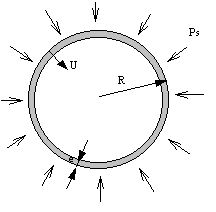
Let \({P}_{s}\) be the confinement pressure defined in the following figure

So we have:

\({P}_{s}\cdot R={\mathrm{\sigma }}_{b}\cdot e\)

If \({k}_{s}=\frac{{K}_{s}}{2\cdot G}\) represents the relative stiffness and \({\lambda }_{d}\) the deconfinement rate when the support is put in place, then the support pressure and the radial displacement in the wall are given by:

\(\{\begin{array}{}{P}_{s}=\frac{{k}_{s}}{1+{k}_{s}}\cdot (1-{\lambda }_{d})\cdot {\sigma }^{0}\\ {U}_{R}=\frac{1+{\lambda }_{d}\cdot {k}_{s}}{1+{k}_{s}}\cdot \frac{{\sigma }^{0}}{2\cdot G}\cdot R\end{array}\)

Summary flow chart on methods to simulate an excavation

Notes

The names of the objects are those of the command files shown in the following appendices.

\(\mathit{SNL}\) means STAT_NON_LINE; \(\mathit{CC}\) means CREA_CHAMP; \(\mathit{CL}\) means boundary conditions

Step 1: Constraint initialization
\(I\): \(\mathit{SNL1}\) with the desired load of its own weight or pressure and a material with a possibly fictitious Poisson’s ratio		\(\mathit{II}\): assignment by command \(\mathit{CC}\) of the desired field
Step 2: Retrieving nodal reactions at the edge of the future gallery
\(\mathit{CC}\) to extract the constraints from \(\mathit{SNL1}\) \(\mathit{SNL}2\) with \(\mathit{CL}\) on the object \(\mathit{BORD}\) in DIDI Retrieving reactions		\(\mathit{SNL}1\) with \(\mathit{CL}\) on object \(\mathit{BORD}\) in DIDIsur model \(\mathit{SOL}\) Retrieving reactions	\(\mathit{SNL}1\) with \(\mathit{CL}\) on object \(\mathit{BORD}\) in DIDIsur model SOL_REST Retrieving reactions
Step 3: End of lockdown
\(\mathit{SNL}3\) with the loading of the nodal reaction vector and a « soft » material in place of the « void »		\(\mathit{SNL}2\) (model \(\mathit{SOL}\)) with the loading of the nodal reactions vector and a « soft » material in place of the « void »	\(\mathit{SNL}2\) (a single material and model SOL_REST) with loading the vector of nodal reactions
Step 4: Installing the support
\(\mathit{SNL}4\) with 3 materials: rock, concrete and void (\(A\) method) to complete the end of lockdown		\(\mathit{SNL}3\) with 3 materials: rock, concrete and void (\(A\) method) to complete the end of lockdown	\(\mathit{CC}\) to extract the results of \(\mathit{SNL}2\) (\(\mathit{SNL}3\)) on a model (SOL_REST + BETON) for intermediate calculation (Combination of fields \(\mathit{CC}\) \(\mathit{SNL}4\)) to complete the end of lockdown

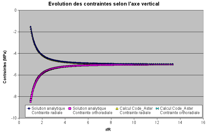
Comparison of the constraints obtained by numerical calculation and by the analytical solution

Unsupported tunnel case

Case of supported tunnels (from 50% of deconfinement)