2. The different steps of a calculation THM#

2.1. Model choice#

Numerical processing in THM requires a quadratic mesh since the elements are of type \(\text{P2}\) in movement and \(\text{P1}\) in pressure and temperature in order to avoid oscillations problems.

The choice is made by using the AFFE_MODELE command as in the example below:

MODELE = AFFE_MODELE (MAILLAGE = MAIL,
                   AFFE =_F (TOUT =' OUI ',
                           PHENOMENE =' MECANIQUE ',
                           MODELISATION =' AXIS_THH2MD ',),
                   )

In all cases, the phenomenon is « MECANIQUE » (even if the modeling does not contain mechanics).

The user must then enter the MODELISATION keyword in a mandatory manner. This keyword allows you to define the type of element assigned to a mesh type. The models available in THM are shown in the following table.

note: Models ending in the letter D indicate that a treatment is being done. allowing the matrix to be diagonalized (« lumper ») in order to avoid oscillations for hydraulic problems. To do this, the integration points are taken at the vertices of the elements. Since this treatment is poorly suited to mechanics, modeling is also available. called « selective ». In this case, the capacitive terms are integrated into the vertices while the Diffusive terms are integrated into Gauss points. These models end with an S. The other models integrate everything at Gauss points.

The user is strongly advised to use D or S models in cases without mechanics and to use S modeling and for modeling with mechanics.

« Classic » models (without D or S) need to be resorbed and are not recommended.

Tableau 2.1 Modélisations THM#
MODELISATION	Geometric modelling	Phenomena taken into account
D_PLAN_HM	plane	Mechanical, hydraulic with unknown pressure. Valid modeling in dynamics
D_PLAN_HMD	plane	Mechanical, hydraulic with unknown pressure (lumped stiffness). Valid modeling in dynamics
D_PLAN_HMS	plane	Mechanical, hydraulic with unknown pressure (selective). Valid modeling in dynamics
D_PLAN_HM_SI	plane	Mechanical, hydraulic with unknown pressure (sub-integrated)
D_PLAN_HHM	plane	Mechanical, hydraulic with two unknown pressures. Valid modeling in dynamics
D_PLAN_HHMD	plane	Mechanical, hydraulic with two unknown pressures (lumped stiffness). Valid modeling in dynamics
D_PLAN_HHMS	plane	Mechanical, hydraulic with two unknown pressures (selective). Valid modeling in dynamics
D_PLAN_HH2MD	plane	Mechanical, hydraulic with two unknown pressures and two components in the gas phase (lumped)
D_PLAN_HH2MS	plane	Mechanical, hydraulic with two unknown pressures and two components in the gas phase (selective)
D_PLAN_HH2M_SI	plane	Mechanical, hydraulic with two unknown pressures and two components in the gas phase (sub-integrated). Valid modeling in dynamics.
D_PLAN_THHD	plane	Thermal, hydraulic with two unknown pressures (lumped)
D_PLAN_THH2D	plane	Thermal, hydraulic with two unknown pressures and two components in the gas phase (lumped)
D_PLAN_THH2S	plane	Thermal, hydraulic with two unknown pressures and two components in the gas phase (selective)
D_PLAN_THM	plane	Thermal, mechanical, hydraulic with unknown pressure. Valid modeling in dynamics
D_PLAN_THVD	plane	Thermal, mechanical, hydraulic with two unknown pressures (2 phases: liquid water and steam) (lumped)
D_PLAN_THMD	plane	Thermal, mechanical, hydraulic with unknown pressure (lumped)
D_PLAN_THMS	plane	Thermal, mechanical, hydraulic with unknown pressure (selective)
D_PLAN_THHMD	plane	Thermal, mechanical, hydraulic with two unknown pressures (lumpé)
D_PLAN_THHMS	plane	Thermal, mechanical, hydraulic with two unknown pressures (selective)
D_PLAN_HHD	plane	hydraulic with two unknown pressures (lumped)
D_PLAN_HHS	plane	hydraulic with two unknown pressures (selective)
D_PLAN_HH2D	plane	hydraulic with two unknown pressures and two components in the gas phase (lumped)
D_PLAN_HH2S	plane	hydraulic with two unknown pressures and two components in the gas phase (selective)
D_PLAN_THH2MD	plan	Thermal, mechanical, hydraulic with two unknown pressures and two components in the gas phase (lumped)
D_PLAN_THH2MS	plane	Thermal, mechanical, hydraulic with two unknown pressures and two components in the gas phase (selective)
AXIS_HM	axisymmetric	Mechanical, hydraulic with unknown pressure. Valid modeling in dynamics
AXIS_HMD	axisymmetric	Mechanical, hydraulic with unknown pressure (lumped stiffness). Valid modeling in dynamics
AXIS_HMS	axisymmetric	Mechanical, hydraulic with unknown pressure (selective). Valid modeling in dynamics
AXIS_HHM	axisymmetric	Mechanical, hydraulic with two unknown pressures. Valid modeling in dynamics
AXIS_HHMD	axisymmetric	Mechanical, hydraulic with two unknown pressures (lumped stiffness). Valid modeling in dynamics
AXIS_HHMS	axisymmetric	Mechanical, hydraulic with two unknown pressures (selective). Valid modeling in dynamics
AXIS_HH2MD	axisymmetric	Mechanical, hydraulic with two unknown pressures and two components in the gas phase (lumped)
AXIS_HH2MS	axisymmetric	Mechanical, hydraulic with two unknown pressures and two components in the gas phase (selective)
AXIS_THHD	axisymmetric	Thermal, hydraulic with two unknown pressures (pumped)
AXIS_THHS	axisymmetric	Thermal, hydraulic with two unknown pressures (selective)
AXIS_THH2D	axisymmetric	Thermal, hydraulic with two unknown pressures and two components in the gas phase (lumped)
AXIS_THH2S	axisymmetric	Thermal, hydraulic with two unknown pressures and two components in the gas phase (selective)
AXIS_THM	axisymmetric	Thermal, mechanical, hydraulic with unknown pressure. Valid modeling in dynamics
AXIS_THMD	axisymmetric	Thermal, mechanical, hydraulic with unknown pressure (pumped)
AXIS_THMS	axisymmetric	Thermal, mechanical, hydraulic with unknown pressure (selective)
AXIS_THVD	axisymmetric	Thermal, mechanical, hydraulic with two unknown pressures (2 phases: liquid water and steam) (lumped)
AXIS_THHMD	axisymmetric	Thermal, mechanical, hydraulic with two unknown pressures (lumped)
AXIS_THHMS	axisymmetric	Thermal, mechanical, hydraulic with two unknown pressures (selective)
AXIS_THH2MD	axisymmetric	Thermal, mechanical, hydraulic with two unknown pressures and two components in the gas phase (lumped)
AXIS_THH2MS	axisymmetric	Thermal, mechanical, hydraulic with two unknown pressures and two components in the gas phase (selective)
AXIS_HHD	axisymmetric	hydraulic with two unknown pressures (pumped)
AXIS_HHS	axisymmetric	hydraulic with two unknown pressures (selective)
AXIS_HH2D	axisymmetric	hydraulic with two unknown pressures and two components in the gas phase (lumped)
AXIS_HH2S	axisymmetric	hydraulic with two unknown pressures and two components in the gas phase (selective)
3D_HM	3D	Mechanical, hydraulic with unknown pressure. Valid modeling in dynamics
3D_HMD	3D	Mechanical, hydraulic with unknown pressure (lumped stiffness). Valid modeling in dynamics
3D_HMS	3D	Mechanical, hydraulic with unknown pressure (selective). Valid modeling in dynamics
3D_HM_SI	3D	Mechanical, hydraulic with unknown pressure (sub-integrated)
3D_HHM	3D	Mechanics, hydraulics with two unknown pressures. Valid modeling in dynamics
3D_HHMD	3D	Mechanical, hydraulic with two unknown pressures (lumped stiffness). Valid modeling in dynamics
3D_HHMS	3D	Mechanical, hydraulic with two unknown pressures (selective). Valid modeling in dynamics
3D_HH2MD	3D	Mechanical, hydraulic with two unknown pressures and two components in the gas phase (lumped)
3D_HH2MS	3D	Mechanical, hydraulic with two unknown pressures and two components in the gas phase (selective)
3D_HH2M_SI	3D	Mechanical, hydraulic with two unknown pressures and two components in the gas phase (sub-integrated). Valid modeling in dynamics.
3D_THHD	3D	Thermal, hydraulic with two unknown pressures (lumped stiffness). Valid modeling in dynamics
3D_THH2D	3D	Thermal, hydraulic with two unknown pressures and two components in the gas phase (lumped)
3D_THH2S	3D	Thermal, hydraulic with two unknown pressures and two components in the gas phase (selective)
3D_THM	3D	Thermal, mechanical, hydraulic with unknown pressure. Valid modeling in dynamics
3D_THMD	3D	Thermal, mechanical, hydraulic with unknown pressure (lumped)
3D_THMS	3D	Thermal, mechanical, hydraulic with unknown pressure (selective)
3D_THVD	3D	Thermal, mechanical, hydraulic with two unknown pressures (2 phases: liquid water and steam) (lumped)
3D_THHM	3D	Thermal, mechanical, hydraulic with two unknown pressures. Valid modeling in dynamics
3D_THHMD	3D	Thermal, mechanical, hydraulic with two unknown pressures (lumpé)
3D_THHMS	3D	Thermal, mechanical, hydraulic with two unknown pressures (selective)
3D_THH2MD	3D	Thermal, mechanical, hydraulic with two unknown pressures and two components in the gas phase (lumped)
3D_THH2MS	3D	Thermal, mechanical, hydraulic with two unknown pressures and two components in the gas phase (selective)
3D_HHD	3D	hydraulic with two unknown pressures (lumped)
3D_HHS	3D	hydraulic with two unknown pressures (selective)
3D_HH2D	3D	hydraulic with two unknown pressures and two components in the gas phase (lumped)
3D_HH2S	3D	hydraulic with two unknown pressures and two components in the gas phase (selective)

The main unknowns, which are also the values of the degrees of freedom, are noted in the case the most complete modeling (thermal, mechanical, hydraulic 3D) with two pressures unknown).

\({\left\{u\right\}}^{\mathrm{ddl}}=\left\{\begin{array}{}{u}_{x}\\ {u}_{y}\\ {u}_{z}\\ {\text{PRE1}}^{\mathrm{ddl}}\\ {\text{PRE2}}^{\mathrm{ddl}}\\ {T}^{\mathrm{ddl}}\end{array}\right\}\)

The content of \(\mathit{PRE1}\) and \(\mathit{PRE2}\) depends on the coupling chosen and will be explained in section 2.2.2.

Depending on the model chosen, only some of these degrees of freedom exist. The table below summarizes the degrees of freedom used for each model.

MODELISATION	\({u}_{x}\)	\({u}_{y}\)		\({u}_{z}\)		\({\mathrm{PRE1}}^{\mathrm{ddl}}\)	\({\mathrm{PRE2}}^{\mathrm{ddl}}\)	\({T}^{\mathrm{ddl}}\)
D_PLAN_HM (_, S, D, SI)	X	X	X	X
D_PLAN_HHM (_, S, D)	X	X	X	X	X
D_PLAN_HH2M (S, D, _SI)	X	X	X	X	X	X
D_PLAN_THH (S, D)					X	X	X
D_PLAN_THH2 (S, D)					X	X	X
D_PLAN_THM (_, S, D)	X	X	X	X		X
D_PLAN_THV (_, S, D)					X	X	X
D_PLAN_THHM (S, D)	X	X	X	X	X	X
D_PLAN_THH2M (S, D)	X	X	X	X	X	X
D_PLAN_HH (S, D)					X	X
D_PLAN_HH2 (S, D)					X	X
AXIS_HM (_, S, D)	X	X		X
AXIS_HHM (_, S, D)	X	X	X	X	X
AXIS_HH2M (S, D)	X	X	X	X	X
AXIS_THH (S, D)					X	X	X
AXIS_THH2 (S, D)					X	X	X
AXIS_THM (_, S, D)	X	X	X	X		X
AXIS_THV (_, S, D)					X	X	X
AXIS_THHM (S, D)	X	X	X	X	X	X
AXIS_THH2M (S, D)	X	X	X	X	X	X
AXIS_HH (S, D)					X	X
AXIS_HH2 (S, D)					X	X
3D_HM (_, S, D, SI)	X	X	X	X
3D_HHM (_, S, D)	X	X	X	X	X	X
3D_HH2M (S, D, _SI)	X	X	X	X	X	X
3D_THH (S, D)					X	X	X
3D_THH2D					X	X	X
3D_THM (_, S, D)	X	X	X	X	X	X
3D_THVD (_, S, D)					X	X	X
3D_THHM (_, S, D)	X	X	X	X	X	X
3D_THH2M (S, D)	X	X	X	X	X	X	X
3D_HH (S, D)					X	X
3D_HH2 (S, D)					X	X

Generalized constraints and internal variables are all shown in [§Annexe 1]. The notations used are those defined in [R7.01.11].

2.2. Definition of material#

The material is defined by the DEFI_MATERIAU command as in the example below:

MATERBO = DEFI_MATERIAU (ELAS = _F (E=5.1500000 0E8, NU=0.20, ALPHA =0.,),
                        COMP_THM = 'LIQU_AD_GAZ_VAPE',
                        THM_LIQU = _F (
                                        RHO =1000.0,
                                        UN_SUR_K =0. ,
                                        ALPHA =0. ,
                                        CP=0.0,
                                        VISC = VISCOLIQ,
                                        D_VISC_TEMP = DVISCOL,
                                        ),
                        THM_GAZ = _F (
                                        MASS_MOL =0.01,
                                        CP=0.0,
                                        VISC = VISCOGAZ,
                                        D_VISC_TEMP = ZERO,
                                        ),
                        THM_VAPE_GAZ = _F (
                                        MASS_MOL =0.01,
                                        CP=0.0,
                                        VISC = VISCOGAZ,
                                        D_VISC_TEMP = ZERO,
                                        ),
                        THM_AIR_DISS = _F (
                                        CP=0.0,
                                        COEF_HENRY = HENRY
                                        ),
                        THM_INIT = _F (
                                        TEMP =300.0,
                                        PRE1 =0.0,
                                        PRE2 =1.E5,
                                        PORO =1. ,
                                        PRES_VAPE =1000.0,
                                        ),
                        THM_DIFFU = _F (
                                        R_GAZ =8.32,
                                        RHO =2200.0,
                                        CP=1000.0,
                                        BIOT_COEF =1.0,
                                        SATU_PRES = SATUBO,
                                        D_SATU_PRES = DSATBO,
                                        PESA_X =0.0,
                                        PESA_Y =0.0,
                                        PESA_Z =0.0,
                                        PERM_IN = KINTBO,
                                        PERM_LIQU = UNDEMI,
                                        D_PERM_LIQU_SATU = ZERO,
                                        PERM_GAZ = UNDEMI,
                                        D_PERM_SATU_GAZ = ZERO,
                                        D_PERM_PRES_GAZ = ZERO,
                                        FICKV_T = ZERO,
                                        FICKA_T = FICK,
                                        LAMB_T = ZERO,
                                        ),
                        )

We are now going to detail each of the keywords. Here we will not focus on the mechanical part — if there is a mechanical part — that depends on the law of behavior chosen. We are For this purpose, refer to the documentation for DEFI_MATERIAU [U4.43.01].

2.2.1. Simple keyword « COMP_THM »#

Allows the coupling law THM to be selected as soon as the material is defined.

GAZ: law of behavior of an ideal gas, i.e. verifying the relationship \(P\mathrm{/}\rho =\mathit{RT}\mathrm{/}\mathit{Mv}\) where \(P\) is pressure, \(\rho\) the density, \(\text{Mv}\) the molar mass, \(R\) the constant of ideal gases and \(T\) the temperature (see [R7.01.11] for more details). For a saturated environment only. The required material field data is provided in the DEFI_MATERIAU operator, under the THM_GAZ keyword.

LIQU_SATU: law of behavior for a porous medium saturated by a single liquid (Cf. [R7.01.11] for more details). The necessary data from the material field are provided in operator DEFI_MATERIAU, under the THM_LIQU keyword.

LIQU_GAZ_ATM: Law of behavior for a porous medium unsaturated with liquid and gas at atmospheric pressure (see [R7.01.11] for more details). The data required for the material field are provided in the DEFI_MATERIAU operator, under the keywords THM_LIQU and THM_GAZ.

LIQU_VAPE_GAZ: law of behavior for an unsaturated porous water/vapour/dry air medium with phase change (see [R7.01.11] for more details). The data required for the material field are provided in the operator DEFI_MATERIAU, under the keywords: THM_LIQU, THM_VAPE, and THM_GAZ.

LIQU_AD_GAZ_VAPE: law of behavior for an unsaturated porous medium water/vapour/dry air/air dissolved with phase change (see [R7.01.11] for more details). Les required data from the material field is provided in operator DEFI_MATERIAU, under keywords THM_LIQU, THM_VAPE, THM_GAZ, and THM_AIR_DISS.

LIQU_AD_GAZ: law of behavior for an unsaturated porous medium water/dry air/dissolved air with phase change (see [R7.01.11] for more details). The data required for the material field are provided in the DEFI_MATERIAU operator, under the keywords THM_LIQU, THM_GAZ, and THM_AIR_DISS.

LIQU_VAPE: law of behavior for a porous medium saturated by a component present in the form liquid or vapor with phase change (see [R7.01.11] for more details). The required material field data is provided in operator DEFI_MATERIAU, under keywords THM_LIQU and THM_VAPE. **This law is only valid for THVD models.

LIQU_GAZ: law of behavior for an unsaturated porous liquid/gas medium with no change in phase (see [R7.01.11] for more details). The required field data material are provided in the DEFI_MATERIAU operator, under the keywords THM_LIQU and THM_GAZ.

The table below summarizes the mandatory keywords for the sub-orders explained in the following sections according to the coupling law chosen.

Legends:	O	Key word required
	T	Mandatory thermal keyword
		Unnecessary keyword for this type of coupling law
	F	Useful for the law but optional (set by default)

+——————————————————–+————-+————+——-+—————-+—————–+——————–+—————+————-++ | |**LIQU_SATU**|**LIQU_GAZ**|**GAZ**|**LIQU_GAZ_ATM**|**LIQU_VAPE_GAZ**|**LIQU_AD_GAZ_VAPE**|**LIQU_AD_GAZ**|**LIQU_VAPE** | +--------------------------------------------------------+-------------+------------+-------+----------------+-----------------+--------------------+---------------+-------------++ |**THM_INIT** |**O** |**O** |**O** |**O** |**O** |**O** |**O** |**O** | +--------------------------------------------------------+-------------+------------+-------+----------------+-----------------+--------------------+---------------+-------------++ |PRE1 |FFFF |FFFF |FFFF |FFFF |FFFF |FFFF |FFFF |FFFF | +--------------------------------------------------------+-------------+------------+-------+----------------+-----------------+--------------------+---------------+-------------++ |PRE2 | |FFFF | | |FFFF |FFFF |FFFF | | +--------------------------------------------------------+-------------+------------+-------+----------------+-----------------+--------------------+---------------+-------------++ |PORO |OOOO |OOOO |OOOO |OOOO |OOOO |OOOO |OOOO |OOOO | +--------------------------------------------------------+-------------+------------+-------+----------------+-----------------+--------------------+---------------+-------------++ |TEMP |FFFF |FFFF |FFFF |FFFF |FFFF |FFFF |FFFF |FFFF | +--------------------------------------------------------+-------------+------------+-------+----------------+-----------------+--------------------+---------------+-------------++ |PRES_VAPE | | | | |OOOO |OOOO |OOOO |OOOO | +--------------------------------------------------------+-------------+------------+-------+----------------+-----------------+--------------------+---------------+-------------++ |**THM_DIFFU** |**O** |**O** |**O** |**O** |**O** |**O** |**O** |**O** | +--------------------------------------------------------+-------------+------------+-------+----------------+-----------------+--------------------+---------------+-------------++ |R_GAZ | |OOOO |OOOO | |OOOO |OOOO |OOOO |OOOO | +--------------------------------------------------------+-------------+------------+-------+----------------+-----------------+--------------------+---------------+-------------++ |RHO |OOOO |OOOO |OOOO |OOOO |OOOO |OOOO |OOOO |OOOO | +--------------------------------------------------------+-------------+------------+-------+----------------+-----------------+--------------------+---------------+-------------++ |BIOT_COEF |OOOO |OOOO |OOOO |OOOO |OOOO |OOOO |OOOO |OOOO | +--------------------------------------------------------+-------------+------------+-------+----------------+-----------------+--------------------+---------------+-------------++ |PESA_X |OOOO |OOOO |OOOO |OOOO |OOOO |OOOO |OOOO |OOOO | +--------------------------------------------------------+-------------+------------+-------+----------------+-----------------+--------------------+---------------+-------------++ |PESA_Y |OOOO |OOOO |OOOO |OOOO |OOOO |OOOO |OOOO |OOOO | +--------------------------------------------------------+-------------+------------+-------+----------------+-----------------+--------------------+---------------+-------------++ |PESA_Z |OOOO |OOOO |OOOO |OOOO |OOOO |OOOO |OOOO |OOOO | +--------------------------------------------------------+-------------+------------+-------+----------------+-----------------+--------------------+---------------+-------------++ |*If law* **HYDR_UTIL** *** (cf. chapter* *) :* || +——————————————————–+————-+————+——-+—————-+—————–+——————–+—————+————-++ |SATU_PRES | |OOOO | |OOOO |OOOO |OOOO |OOOO |OOOO | +--------------------------------------------------------+-------------+------------+-------+----------------+-----------------+--------------------+---------------+-------------++ |D_SATU_PRES | |OOOO | |OOOO |OOOO |OOOO |OOOO |OOOO | +--------------------------------------------------------+-------------+------------+-------+----------------+-----------------+--------------------+---------------+-------------++ |PERM_LIQU | |OOOO | |OOOO |OOOO |OOOO |OOOO |OOOO | +--------------------------------------------------------+-------------+------------+-------+----------------+-----------------+--------------------+---------------+-------------++ |D_PERM_LIQU_SATU | |OOOO | |OOOO |OOOO |OOOO |OOOO |OOOO | +--------------------------------------------------------+-------------+------------+-------+----------------+-----------------+--------------------+---------------+-------------++ |PERM_GAZ | |OOOO | | |OOOO |OOOO |OOOO |OOOO | +--------------------------------------------------------+-------------+------------+-------+----------------+-----------------+--------------------+---------------+-------------++ |D_PERM_SATU_GAZ | |OOOO | | |OOOO |OOOO |OOOO |OOOO | +--------------------------------------------------------+-------------+------------+-------+----------------+-----------------+--------------------+---------------+-------------++ |D_PERM_PRES_GAZ | |OOOO | | |OOOO |OOOO |OOOO |OOOO | +--------------------------------------------------------+-------------+------------+-------+----------------+-----------------+--------------------+---------------+-------------++ |*If law* **HYDR_VGM** *or HYDR_VGC (cf.* *section* *) :* || +——————————————————–+————-+————+——-+—————-+—————–+——————–+—————+————-++ |VG_N | |OOOO | | |OOOO |OOOO |OOOO | | +--------------------------------------------------------+-------------+------------+-------+----------------+-----------------+--------------------+---------------+-------------++ |VG_PR | |OOOO | | |OOOO |OOOO |OOOO | | +--------------------------------------------------------+-------------+------------+-------+----------------+-----------------+--------------------+---------------+-------------++ |VG_SR | |OOOO | | |OOOO |OOOO |OOOO | | +--------------------------------------------------------+-------------+------------+-------+----------------+-----------------+--------------------+---------------+-------------++ |VG_SMAX | |OOOO | | |OOOO |OOOO |OOOO | | +--------------------------------------------------------+-------------+------------+-------+----------------+-----------------+--------------------+---------------+-------------++ |VG_SATUR | |OOOO | | |OOOO |OOOO |OOOO | | +--------------------------------------------------------+-------------+------------+-------+----------------+-----------------+--------------------+---------------+-------------++ |*If law* **HYDR_** TABBAL *(cf.* *section* *) :* | +--------------------------------------------------------+-------------+------------+-------+----------------+-----------------+--------------------+---------------+-------------++ |SATU_PRES | |OOOO | |OOOO |OOOO |OOOO |OOOO |OOOO | +--------------------------------------------------------+-------------+------------+-------+----------------+-----------------+--------------------+---------------+-------------++ |D_SATU_PRES | |OOOO | |OOOO |OOOO |OOOO |OOOO |OOOO | +--------------------------------------------------------+-------------+------------+-------+----------------+-----------------+--------------------+---------------+-------------++ |PERM_LIQU | |OOOO | |OOOO |OOOO |OOOO |OOOO |OOOO | +--------------------------------------------------------+-------------+------------+-------+----------------+-----------------+--------------------+---------------+-------------++ |D_PERM_LIQU_SATU | |OOOO | |OOOO |OOOO |OOOO |OOOO |OOOO | +--------------------------------------------------------+-------------+------------+-------+----------------+-----------------+--------------------+---------------+-------------++ |PERM_GAZ | |OOOO | | |OOOO |OOOO |OOOO |OOOO | +--------------------------------------------------------+-------------+------------+-------+----------------+-----------------+--------------------+---------------+-------------++ |D_PERM_SATU_GAZ | |OOOO | | |OOOO |OOOO |OOOO |OOOO | +--------------------------------------------------------+-------------+------------+-------+----------------+-----------------+--------------------+---------------+-------------++ |D_PERM_PRES_GAZ | |OOOO | | |OOOO |OOOO |OOOO |OOOO | +--------------------------------------------------------+-------------+------------+-------+----------------+-----------------+--------------------+---------------+-------------++ |EPAI | |OOOO | | |OOOO |OOOO |OOOO | | +--------------------------------------------------------+-------------+------------+-------+----------------+-----------------+--------------------+---------------+-------------++ |A0 | |OOOO | | |OOOO |OOOO |OOOO | | +--------------------------------------------------------+-------------+------------+-------+----------------+-----------------+--------------------+---------------+-------------++ |SHUTTLE | |OOOO | | |OOOO |OOOO |OOOO | | +--------------------------------------------------------+-------------+------------+-------+----------------+-----------------+--------------------+---------------+-------------++ |S_BJH | |OOOO | | |OOOO |OOOO |OOOO | | +--------------------------------------------------------+-------------+------------+-------+----------------+-----------------+--------------------+---------------+-------------++ |W_BJH | |OOOO | | |OOOO |OOOO |OOOO | | +--------------------------------------------------------+-------------+------------+-------+----------------+-----------------+--------------------+---------------+-------------++ | || +——————————————————–+————-+————+——-+—————-+—————–+——————–+—————+————-++ |FICKV_T | | | | |OOOO |OOOO | | | +——————————————————–+————-+————+——-+—————-+—————–+——————–+—————+————-++ |FICKV_PV | | | | |FFFF |FFFF | | | +——————————————————–+————-+————+——-+—————-+—————–+——————–+—————+————-++ |FICKV_PG | | | | |FFFF |FFFF | | | +——————————————————–+————-+————+——-+—————-+—————–+——————–+—————+————-++ |FICKV_S | | | | |FFFF |FFFF | | | +——————————————————–+————-+————+——-+—————-+—————–+——————–+—————+————-++ |D_FV_T | | | | |FFFF |FFFF | | | +——————————————————–+————-+————+——-+—————-+—————–+——————–+—————+————-++ |D_FV_PG | | | | |FFFF |FFFF | | | +——————————————————–+————-+————+——-+—————-+—————–+——————–+—————+————-++ |FICKA_T | | | | | |OOOO |OOOO | | +——————————————————–+————-+————+——-+—————-+—————–+——————–+—————+————-++ |FICKA_PA | | | | | |FFFF |FFFF | | +——————————————————–+————-+————+——-+—————-+—————–+——————–+—————+————-++ |FICKA_PL | | | | | |FFFF |FFFF | | +——————————————————–+————-+————+——-+—————-+—————–+——————–+—————+————-++ |FICKA_S | | | | | |FFFF |FFFF | | +——————————————————–+————-+————+——-+—————-+—————–+——————–+—————+————-++ |D_FA_T | | | | | |FFFF |FFFF | | +——————————————————–+————-+————+——-+—————-+—————–+——————–+—————+————-++ |CP |TTTT |TTTT |TTTT |TTTT |TTTT |TTTT |TTTT |TTTT | +——————————————————–+————-+————+——-+—————-+—————–+——————–+—————+————-++ |PERM_IN/PERM_END/PERM_L, PERM_N, PERM_T |OOOO |OOOO |OOOO |OOOO |OOOO |OOOO |OOOO |OOOO | +——————————————————–+————-+————+——-+—————-+—————–+——————–+—————+————-++ |LAMB_T/LAMB_TL, LAMB_TN, LAMB_TT |TTTT |TTTT |TTTT |TTTT |TTTT |TTTT |TTTT |TTTT | +——————————————————–+————-+————+——-+—————-+—————–+——————–+—————+————-++ |LAMB_S | | | | | | | | | +——————————————————–+————-+————+——-+—————-+—————–+——————–+—————+————-++ |LAMB_PHI | | | | | | | | | +——————————————————–+————-+————+——-+—————-+—————–+——————–+—————+————-++ |LAMB_CT/LAMB_C_L, LAMB_C_N, LAMB_C_T | | | | | | | | | +——————————————————–+————-+————+——-+—————-+—————–+——————–+—————+————-++ |D_LB_T/D_LB_TT, D_LB_TL, D_LB_T, | | | | | | | | | +——————————————————–+————-+————+——-+—————-+—————–+——————–+—————+————-++ |D_LB_S | | | | | | | | | +——————————————————–+————-+————+——-+—————-+—————–+——————–+—————+————-++ |D_LB_PHI | | | | | | | | | +——————————————————–+————-+————+——-+—————-+—————–+——————–+—————+————-++ |THM_LIQU |O |O | |O |O |O |O |O | +——————————————————–+————-+————+——-+—————-+—————–+——————–+—————+————-++ |RHO |OOOO |OOOO | |OOOO |OOOO |OOOO |OOOO |OOOO | +——————————————————–+————-+————+——-+—————-+—————–+——————–+—————+————-++ |UN_SUR_K |OOOO |OOOO | |OOOO |OOOO |OOOO |OOOO |OOOO | +——————————————————–+————-+————+——-+—————-+—————–+——————–+—————+————-++ |VISC |OOOO |OOOO | |OOOO |OOOO |OOOO |OOOO |OOOO | +——————————————————–+————-+————+——-+—————-+—————–+——————–+—————+————-++ |D_VISC_TEMP |OOOO |OOOO | |OOOO |OOOO |OOOO |OOOO |OOOO | +——————————————————–+————-+————+——-+—————-+—————–+——————–+—————+————-++ |ALPHA |TTTT |TTTT | |TTTT |TTTT |TTTT |TTTT |TTTT | +——————————————————–+————-+————+——-+—————-+—————–+——————–+—————+————-++ |CP |TTTT |TTTT | |TTTT |TTTT |TTTT |TTTT |TTTT | +——————————————————–+————-+————+——-+—————-+—————–+——————–+—————+————-++ |THM_GAZ | |O |O |O |O |O |O | | +——————————————————–+————-+————+——-+—————-+—————–+——————–+—————+————-++ |MASS_MOL | |OOOO |OOOO |OOOO |OOOO |OOOO |OOOO | | +——————————————————–+————-+————+——-+—————-+—————–+——————–+—————+————-++ |VISC | |OOOO |OOOO |OOOO |OOOO |OOOO |OOOO | | +——————————————————–+————-+————+——-+—————-+—————–+——————–+—————+————-++ |D_VISC_TEMP | |OOOO |OOOO |OOOO |OOOO |OOOO |OOOO | | +——————————————————–+————-+————+——-+—————-+—————–+——————–+—————+————-++ |CP | |TTTT |TTTT |TTTT |TTTT |TTTT |TTTT | | +——————————————————–+————-+————+——-+—————-+—————–+——————–+—————+————-++ |THM_VAPE_GAZ | | | | |O |O | |O | +——————————————————–+————-+————+——-+—————-+—————–+——————–+—————+————-++ |MASS_MOL | | | | |OOOO |OOOO | |OOOO | +——————————————————–+————-+————+——-+—————-+—————–+——————–+—————+————-++ |CP | | | | |OOOO |OOOO | |OOOO | +——————————————————–+————-+————+——-+—————-+—————–+——————–+—————+————-++ |VISC | | | | |OOOO |OOOO | |OOOO | +——————————————————–+————-+————+——-+—————-+—————–+——————–+—————+————-++ |D_VISC_TEMP | | | | |OOOO |OOOO | |OOOO | +——————————————————–+————-+————+——-+—————-+—————–+——————–+—————+————-++ |THM_AIR_DISS | | | | | |O |O | | +——————————————————–+————-+————+——-+—————-+—————–+——————–+—————+————-++ |CP | | | | | |OOOO |OOOO | | +——————————————————–+————-+————+——-+—————-+—————–+——————–+—————+————-++ |COEF_HENRY | | | | | |OOOO |OOOO | | +——————————————————–+————-+————+——-+—————-+—————–+——————–+—————+————-++

The table below summarizes the compatibility between the laws of behavior and the models chosen:

MODELISATION	Authorized law of hydraulic behavior
_HM (_, S, D, YES)	LIQU_SATU, GAZ, LIQU_GAZ_ATM
_ HHM (_, S, D)	LIQU_GAZ, LIQU_VAPE_GAZ
_ HH2M (S, D, _SI)	LIQU_AD_GAZ, LIQU_AD_GAZ_VAPE
_ THH (S, D)	LIQU_GAZ, LIQU_VAPE_GAZ
_ THH2 (S, D)	LIQU_AD_GAZ, LIQU_AD_GAZ_VAPE
_ THM (_, S, D)	LIQU_SATU, GAZ, LIQU_GAZ_ATM
_ THV (_, S, D)	LIQU_VAPE
_ THHM (S, D)	LIQU_GAZ, LIQU_VAPE_GAZ
_ THH2M (S, D)	LIQU_AD_GAZ, LIQU_AD_GAZ_VAPE
_HH (S, D)	LIQU_GAZ, LIQU_VAPE_GAZ
_ HH2 (S, D)	LIQU_AD_GAZ, LIQU_AD_GAZ_VAPE

2.2.2. Keyword factor THM_INIT#

For all Thermo-Hydro-Mechanical behaviors, it makes it possible to describe a reference state of the structure (cf. [R7.01.10] and [R7.01.11]).

Under this keyword, there are three quantities corresponding to degrees of freedom. To fully understand These data, we must then distinguish the unknowns at the nodes, which we call \({\left\{u\right\}}^{\text{ddl}}\) and the values defined under the THM_INIT keyword that we Let’s call \({p}^{\text{ref}}\) and \({T}^{\text{ref}}\)

\({\left\{u\right\}}^{\text{ddl}}=\left\{\begin{array}{}{u}_{x}\\ {u}_{y}\\ {u}_{z}\\ {\text{PRE1}}^{\text{ddl}}\\ {\text{PRE2}}^{\text{ddl}}\\ {T}^{\text{ddl}}\end{array}\right\}\)

The meaning of the unknowns PRE1 and PRE2 varies between models. Noting \({p}_{w}\) water pressure, \({p}_{\text{ad}}\) dissolved air pressure, \({p}_{\text{lq}}\) liquid pressure \({p}_{\text{lq}}={p}_{w}+{p}_{\text{ad}}\), \({p}_{\text{as}}\), \({p}_{\text{vp}}\) the vapour pressure, \({p}_{\text{as}}\) the dry air pressure and \({p}_{g}={p}_{\text{as}}+{p}_{\text{vp}}\) the total gas pressure and \({p}_{c}={p}_{g}-{p}_{\text{lq}}\) capillary pressure (also called suction), we have the The following meanings of unknowns PRE1 and PRE2

Tableau 2.2 contenu de PRE1 et PRE2#
Behavior KIT	LIQU_SATU	LIQU_GAZ_ATM	GAZ	LIQU_VAPE_GAZ
\(\mathit{PRE1}\)	\({p}_{\text{lq}}\)	\(-{p}_{\text{lq}}\)		\({p}_{g}\)	\({p}_{c}={p}_{g}-{p}_{\text{lq}}\)
\(\mathit{PRE2}\)				\({p}_{g}\)

Tableau 2.3 contenu de PRE1 et PRE2#
Behavior KIT	LIQU_GAZ	LIQU_VAPE	LIQU_AD_GAZ_VAPE or LIQU_AD_GAZ
\(\mathit{PRE1}\)	\({p}_{c}={p}_{g}-{p}_{\text{lq}}\)	\({p}_{\text{lq}}\)	\({p}_{c}={p}_{g}-{p}_{\text{lq}}\)
\(\mathit{PRE2}\)	\({p}_{g}\)		\({p}_{g}\)

The « total » pressures and temperature are then defined by:

\(p={p}^{\text{ddl}}+{p}^{\text{ref}};T={T}^{\text{ddl}}+{T}^{\text{ref}}\)

All input or output values (boundary conditions or the result of IMPR_RESU) are the nodal unknowns \({p}^{\text{ddl}}\text{et}{T}^{\text{ddl}}\).

On the other hand, it is the pressures and the total temperature that are used in the laws of behavior \(\frac{p}{\rho }=\frac{R}{M}T\) for ideal gases, \(\frac{d{\rho }_{l}}{{\rho }_{l}}=\frac{{\mathrm{dp}}_{l}}{{K}_{l}}-3{\alpha }_{l}\mathrm{dT}\) for liquid and in the saturation/capillary pressure relationship.

We can therefore choose to initialize the nodal values in THM_INIT (by default) these values. are null) or by the ETAT_INIT keyword from the STAT_NON_LINE command or by a combination of two (this can allow easy conversion from Kelvin to degrees Celsius for example).

TEMP is the \({T}_{\text{ref}}\) reference temperature. By default it is taken equal to zero. Attention the initial temperature value \(T={T}^{\text{ddl}}+{T}^{\text{ref}}\) must be strictly greater than zero.

PRE1 is taken to be zero by default. As seen in the table:

For behaviors LIQU_SATU, and LIQU_VAPE this is the reference liquid pressure.
For behavior GAZ this is the reference gas pressure. In this case, the initial pressure of gas \(p={p}^{\text{ddl}}+{p}^{\text{ref}}\) must be non-zero.
For behavior LIQU_GAZ_ATM it’s the reference liquid pressure changed sign.
For behaviors LIQU_VAPE_GAZ, LIQU_AD_GAZ, LIQU_AD_GAZ_VAPE, and LIQU_GAZ this is reference capillary pressure.

PRE2 is taken to be zero by default. For behaviors LIQU_VAPE_GAZ, LIQU_AD_GAZ, LIQU_AD_GAZ_VAPE and LIQU_GAZ are the reference gas pressure. The initial pressure of gas \(p={p}^{\text{ddl}}+{p}^{\text{ref}}\) must be non-zero.

PORO is the initial porosity.

PRES_VAPE is the reference vapour pressure for LIQU_VAPE_GAZ behaviors, LIQU_AD_GAZ_VAPE and LIQU_VAPE.

notes

The initial vapour pressure should be taken in accordance with the other data. Well often, we start from knowing an initial state of humidity. The hygrometric degree Is the ratio between the vapour pressure and the saturating vapour pressure at temperature considered. We then use Kelvin’s law which gives the pressure of the liquid as a function of vapour pressure, temperature and saturating vapour pressure:

\[\frac{{p}_{w}{-}{p}_{w}^{\text{ref}}}{{\rho }_{w}} = \frac{R}{{M}_{\mathit{vp}}^{\mathit{ol}}}T\mathrm{ln}(\frac{{p}_{\mathit{vp}}}{{p}_{\mathit{vp}}^{\mathit{sat}}(T)})\]

This relationship is only valid for isothermal evolutions. It is emphasized that \({p}_{w}^{\text{ref}}\) corresponds to a state of balance to which corresponds \({p}_{\mathit{pv}}^{\mathit{sat}}\), this state of balance actually corresponds to \({p}_{w}^{0}={p}_{\mathit{gz}}^{0}=1\mathit{atm}\). For evolutions with temperature variation, knowing a law giving the pressure of saturating steam at temperature \({T}_{0}\), for example

\[{p}_{\mathit{pv}}^{\mathit{sat}}({T}_{0}) = {10}^{(2.7858+\frac{{T}_{0}{-}273.5}{31.559+0.1354({T}_{0}{-}273.5)})}\]

and a humidity level \(\mathit{HR}\), the vapor pressure is deduced from this thanks to \({p}_{\mathit{pv}}({T}_{0})=\mathit{HR}{p}_{\mathit{pv}}^{\mathit{sat}}({T}_{0})\). Also, you should never take a value of PRES_VAPE equal to zero.

2.2.3. Keyword factor THM_LIQU#

This key word concerns all THM behaviors involving liquid (cf. [R7.01.11]).

RHO is the initial density of the liquid.

UN_SUR_K is the opposite of liquid compressibility: \({K}_{l}\).

VISC is the viscosity of the liquid. Temperature function.

D_VISC_TEMP is the derivative of the viscosity of the liquid with respect to temperature, a function of the temperature. The user must ensure consistency with the function associated with the VISC keyword.

ALPHA is the expansion coefficient (linear) of liquid \({\alpha }_{l}\)

If \({p}_{l}\) refers to the pressure of the liquid, \({\rho }_{l}\) its density and \(T\) the temperature, the behavior of the liquid is

\[\frac{{\mathrm{d\rho }}_{l}}{{\rho }_{l}}=\frac{{\text{dp}}_{l}}{{K}_{l}}-3{\alpha }_{l}\text{dT}\]

CP is the specific heat at constant pressure of the liquid.

2.2.4. Keyword factor THM_GAZ#

This key word factor concerns all THM behaviors involving gas (cf. [R7.01.11]). For behaviors involving both liquid and gas, and when taking Taking into account the evaporation of the liquid, the coefficients given here refer to dry gas. properties of steam will be specified under the keyword THM_VAPE_GAZ.

MASS_MOL is the molar mass of dry gas \({M}_{\text{gs}}\)

If \({p}_{\text{gs}}\) refers to the pressure of dry gas, \({\rho }_{\mathrm{gs}}\) its mass by volume, \(R\) the ideal gas constant and \(T\) the temperature, The behavior of dry gas is

\[\frac{{p}_{\text{gs}}}{{\rho }_{\text{gs}}}=\frac{\text{RT}}{{M}_{\text{gs}}}\]

CP is the specific heat at constant pressure of dry gas.

VISC is the viscosity of dry gas. A function of temperature.

D_VISC_TEMP is the derivative of the viscosity of dry gas with respect to temperature. Function of temperature, the user must ensure consistency with the function associated with VISC.

2.2.5. Keyword factor THM_VAPE_GAZ#

This keyword factor concerns all THM behaviors involving both liquid and a gas, and taking into account the evaporation of the liquid (cf. [R7.01.11]). The coefficients given here refer to steam.

MASS_MOL is the molar mass of steam. \({M}_{\text{vp}}\)

CP is the specific heat at constant pressure of steam.

VISC is the viscosity of the vapor. Temperature function.

D_VISC_TEMP is the derivative of the viscosity of steam with respect to temperature. Function of the temperature. The user must ensure consistency with the function associated with VISC.

2.2.6. Keyword factor THM_AIR_DISS#

This keyword factor is about behavior THM THM_AIR_DISS taking into account the dissolution of the air in the liquid (cf. [R7.01.11]). The coefficients entered here relate to dissolved air.

CP is the specific heat at constant pressure of dissolved air.

COEF_HENRY is Henry’s constant \({K}_{H}\), making it possible to relate the molar concentration of dissolved air \({C}_{\text{ad}}^{\text{ol}}\) (\(\mathit{moles}\mathrm{/}{m}^{3}\)) at air pressure Dry: \({C}_{\text{ad}}^{\text{ol}}=\frac{{p}_{\text{as}}}{{K}_{H}}\)

note: The Henry constant we are using here is expressed in \(\mathit{Pa.}{m}^{3}.{\mathit{mol}}^{{-}1}\). In literature there are various ways to write Henry’s law. For example in Andra’s benchmarks, Henry’s law is given by \({\omega }_{l}^{a}=\frac{{P}_{\text{as}}}{H}\frac{{M}_{\text{as}}^{\text{ol}}}{{M}_{w}}{\rho }_{w}\) with the concentration of air in water that can be reduced to a density such as \({\omega }_{l}^{a}={\rho }_{\text{ad}}\). \(H\) is a coefficient that is expressed in \(\mathit{Pa}\). In these cases, you will have to write the equivalence \({K}_{H}=H\frac{{M}_{w}}{{\rho }_{w}}\)

2.2.7. Keyword factor THM_DIFFU#

This factor keyword is mandatory for all THM behaviors (cf. [R7.01.11]). The user must ensure the consistency of the functions and their derivatives.

note: For orthotropy, the user has several possibilities: place himself in an isotropic framework classical or to be placed in a case of transverse isotropy in 3D. In this case he will have to fill in a certain number of material data (see below) in the L and N directions of the orthotropy coordinate system, the L coordinate system, T being the isotropy coordinate system (cf. R4.01.02). In the case 2D, the concept of transverse isotropy loses its meaning and only in this case, we place ourselves in an orthotropic frame. For the elastic mechanical part, reference will be made to R4.01.02 and the 3 directions will have to be taken into account. For the terms conducting (hydraulic) and thermal), only the directions L and T of the plane will be entered this time (corresponding to the X, Y coordinate system (if the global coordinate system coincides with the local coordinate system).

Careful! Anisotropy in mechanics is only valid for elastic mechanical behavior (not programmed for other laws).

♦ R_GAZ

Ideal gas constant.

♦ RHO

For hydraulic behaviors initial homogenized density [R7.01.11]. It is the one that will be involved in the momentum balance equation and in the hydraulic part. Attention in cases with dynamics and only in these cases, it will also be necessary to enter the density in « ELAS » which will be used for inertia forces (the user must therefore take care to be consistent between these two values).

◊ CP

For thermal behaviors, specific heat with constant stress of the solid alone (grains).

Note:

Attention, this is specific heat only and not « \(\rho {C}_{p}\) », as is done for other thermal controls. The density of the grains is calculated in the code from the homogenized density [R7.01.11].

♦ BIOT_COEF

Biot coefficient used in the isotropic case.

♦ BIOT_L, BIOT_N

In the transverse isotropic case (3D only), the Biot coefficients for the directions L and N of the local orthotropy coordinate system. In this case both are mandatory.

♦ BIOT_L, BIOT_N, BIOT_T

In the orthotropic case (in 2D only), the Biot coefficients for the L and N T directions. In this case all three are mandatory.

♦ PESA_X, PESA_Y, PESA_Z

Gravity according to x, y and z

Note:

The gravity defined here is that used in the Darcy equation only. When there are mechanical calculations, gravity is also defined in * AFFE_CHAR_MECA .This remark applies of course for all three components of gravity.

◊ PERM_IN [function**]

Intrinsic permeability as a function of porosity in the isotropic case.

Permeability in the classical sense \(K\), whose dimension is that of a speed, is calculated as follows:

\(K=\frac{{K}_{\text{int}}{K}_{\text{rel}}}{m}{\rho }_{l}g\) where \({K}_{\text{int}}\) is the intrinsic permeability, \({K}_{\text{rel}}\) the relative permeability, the relative permeability, \(m\) the viscosity, \({\rho }_{l}\) the density of the liquid and \(g\) the acceleration of gravity. Mandatory in the isotropic case.

◊ PERMIN_L, PERMIN_N [function**]

In the 3D transverse isotropic case, the intrinsic permeability for the L and N directions of the local orthotropy coordinate system. In this case both are mandatory.

◊ PERMIN_L, PERMIN_T [function**]

In the orthotropic case in 2D, the intrinsic permeability for the L and T directions of the local coordinate system (corresponding to X, Y without angle rotation). In this case both are mandatory.

◊ SATU_PRES [function**]

For the behaviors of unsaturated materials (LIQU_VAPE_GAZ, LIQU_VAPE, LIQU_GAZ,,,,, LIQU_GAZ_ATM,, LIQU_AD_GAZ, LIQU_AD_GAZ_VAPE), saturation isotherm as a function of capillary pressure. Only for coupling laws HYDR_UTIL, HYDR_TABBAL or HYDR_ENDO (see section 2.5). It is also possible to specify several isotherms depending on the temperature by then using DEFI_NAPPE (in the case HYDR_UTIL).

note: For numerical reasons, it is necessary to avoid saturation reaching the value 1. Also he It is very strongly recommended to multiply capillary function (generally understood). between 0. and 1.) by 0.999.

◊ D_SATU_PRES [function**]

For the behaviors of unsaturated materials (LIQU_VAPE_GAZ, LIQU_VAPE, LIQU_GAZ,,,,, LIQU_GAZ_ATM,, LIQU_AD_GAZ, LIQU_AD_GAZ_VAPE), derived from saturation with respect to pressure. Only for the coupling laws « HYDR_UTIL », « HYDR_TABBAL » or « » or « HYDR_ENDO » (see section 2.5). In addition, several derivatives of the different isotherms depending on the temperature can be entered using « DEFI_NAPPE » [U4.31.03] then using « » [] (in the case « HYDR_UTIL ») (in the case « « ).

◊ PERM_LIQ [function**]

For the behaviors of unsaturated materials (LIQU_VAPE_GAZ, LIQU_VAPE, LIQU_GAZ,,,,, LIQU_GAZ_ATM,, LIQU_AD_GAZ, LIQU_AD_GAZ_VAPE), relative liquid permeability: a function of saturation. Only for the « HYDR_UTIL », « HYDR_TABBAL », or « HYDR_ENDO » coupling laws (see section 2.5).

◊ D_PERM_LIQ_SATU [function**]

For the behaviors of unsaturated materials (LIQU_VAPE_GAZ, LIQU_VAPE, LIQU_GAZ,,,, LIQU_GAZ_ATM,,, LIQU_AD_GAZ, LIQU_AD_GAZ_VAPE), derived from the relative permeability to liquid with respect to saturation: a function of saturation. Only for the « HYDR_UTIL », « HYDR_TABBAL », or « HYDR_ENDO » coupling laws (see section 2.5).

◊ PERM_GAZ [function**]

For the behaviors of unsaturated materials (LIQU_VAPE_GAZ, LIQU_VAPE,,, LIQU_GAZ,, LIQU_AD_GAZ, LIQU_AD_GAZ_VAPE), relative gas permeability: a function of gas saturation and pressure. Only for coupling laws HYDR_UTIL, HYDR_TABBAL or HYDR_ENDO (see section 2.5).

◊ D_PERM_SATU_GAZ [function**]

For the behaviors of unsaturated materials (LIQU_VAPE_GAZ, LIQU_VAPE,,, LIQU_GAZ,, LIQU_AD_GAZ, LIQU_AD_GAZ_VAPE), derived from gas permeability in relation to saturation: a function of gas saturation and pressure. Only for the « HYDR_UTIL », « HYDR_TABBAL », or « HYDR_ENDO » coupling laws (see section 2.5).

◊ D_PERM_PRES_GAZ [function**]

For the behaviors of unsaturated materials (LIQU_VAPE_GAZ, LIQU_VAPE, LIQU_GAZ,,, LIQU_AD_GAZ, LIQU_AD_GAZ_VAPE), derived from gas permeability in relation to gas pressure: a function of saturation and gas pressure. Only for the « HYDR_UTIL », « HYDR_TABBAL », or « HYDR_ENDO » coupling laws (see section 2.5).

◊ VG_N [I]

For the behaviors of unsaturated materials with two unknowns (LIQU_VAPE_GAZ, LIQU_AD_GAZ,, LIQU_AD_GAZ_VAPE, LIQU_GAZ) and in the case where the hydraulic law is « HYDR_VGM » or « HYDR_VGC » (see section 2.5), designate the parameter \(N\) of the Mualem Van-Genuchten law used to define capillary pressure and permeabilities relating to water and gas.

◊ VG_PR [R]

For the behaviors of unsaturated materials with two unknowns (LIQU_VAPE_GAZ, LIQU_AD_GAZ,, LIQU_AD_GAZ_VAPE, LIQU_GAZ) and in the case where the hydraulic law is « HYDR_VGM » or « HYDR_VGC » (see section 2.5), designate the parameter \(\mathit{Pr}\) of the Mualem Van-Genuchten law used to define capillary pressure and permeabilities relating to water and gas.

◊ VG_SR [R]

For the behaviors of unsaturated materials with two unknowns (LIQU_VAPE_GAZ, LIQU_AD_GAZ,, LIQU_AD_GAZ_VAPE, LIQU_GAZ) and in the case where the hydraulic law is HYDR_VGM or HYDR_VGC (see section 2.5), designate the residual saturation parameter \(\mathit{Sr}\) of the Mualem Van-Genuchten law used to define capillary pressure and permeabilities relating to water and gas.

◊ VG_PENTR [R]

For the behaviors of unsaturated materials with two unknowns (LIQU_VAPE_GAZ, LIQU_AD_GAZ,, LIQU_AD_GAZ_VAPE, LIQU_GAZ) and in the case where the hydraulic law is HYDR_VGM or HYDR_VGC (see section 2.5), designate the input pressure parameter \({P}_{e}\) from the Mualem Van-Genuchten law. The medium only desaturates when the capillary pressure is greater than this value (0. by default).

◊ VG_SMAX [R]

For the behaviors of unsaturated materials with two unknowns (LIQU_VAPE_GAZ, LIQU_AD_GAZ,, LIQU_AD_GAZ_VAPE, LIQU_GAZ) and in the case where the hydraulic law is « HYDR_VGM » or « HYDR_VGC » (see section 2.5), designate the maximum saturation for which the Mualem Van-Genuchten law is applied. Beyond this saturation, the Mualem-Van Genuchten curves are interpolated. This value should be very close to 1.

◊ VG_SATUR [R]

For the behaviors of unsaturated materials with two unknowns (LIQU_VAPE_GAZ, LIQU_AD_GAZ,,, LIQU_AD_GAZ_VAPE, LIQU_GAZ) and in the case where the hydraulic law is « HYDR_VGM » or « HYDR_VGC » (see section 2.5). Beyond the saturation defined by « VG_SMAX », the saturation is multiplied by this corrective factor. This value must be very close to 1 (see doc. [R7.01.11]).

◊ EPAI [function**]

2.5

For the behaviors of unsaturated materials with two unknowns (LIQU_VAPE_GAZ, LIQU_AD_GAZ,,,, LIQU_AD_GAZ_VAPE,,, LIQU_GAZ, LIQU_GAZ_ATM) and in the case where the hydraulic law is HYDR_TABBAL (see section). This function refers to the thickness of the adsorbed layer \(t(\mathit{HR})\) which can be determined by an empirical law of Badmann [2] (See Appendix).

◊ A0 [R]

2.5

For the behaviors of unsaturated materials with two unknowns (LIQU_VAPE_GAZ, LIQU_AD_GAZ,,,, LIQU_AD_GAZ_VAPE,,, LIQU_GAZ, LIQU_GAZ_ATM) and in the case where the hydraulic law is HYDR_TABBAL (see section). This parameter refers to the total surface area of the pores (or specific surface area of the material) per unit volume. It is determined by a calculation BET [4] or BJH [3] (See Appendix)

◊ SHUTTLE [R]

2.5

For the behaviors of unsaturated materials with two unknowns (LIQU_VAPE_GAZ, LIQU_AD_GAZ, LIQU_AD_GAZ_VAPE, LIQU_GAZ, LIQU_GAZ_ATM) and in the case where the hydraulic law is HYDR_TABBAL (see section). This parameter refers to a term from Shuttleworth’s law.:math: {left (frac {partialgamma} {partial {epsilon} _ {s}}right) |} _ {mu}) |} _ {mu} `, it can be adjusted to experimental drying shrinkage data (See Appendix).

◊ S_BJH [function**]

2.5

For the behaviors of unsaturated materials with two unknowns (LIQU_VAPE_GAZ, LIQU_AD_GAZ,,,, LIQU_AD_GAZ_VAPE,,, LIQU_GAZ, LIQU_GAZ_ATM) and in the case where the hydraulic law is « HYDR_TABBAL » (see section). This function refers to the volume fraction of liquid water \({S}_{\mathit{BJH}}\) as a function of HR, determined by the BJH [3] method (See Appendix).

◊ W_BJH [function**]

2.5

For the behaviors of unsaturated materials with two unknowns (LIQU_VAPE_GAZ, LIQU_AD_GAZ,,,, LIQU_AD_GAZ_VAPE,,, LIQU_GAZ, LIQU_GAZ_ATM) and in the case where the hydraulic law is HYDR_TABBAL (see section). This function refers to the volume fraction of unsaturated pores \({\mathrm{\omega }}_{\mathit{BJH}}\) as a function of HR, determined by the BJH [3] method (See Appendix).

◊ FICKV_T [function**]

For behaviors LIQU_VAPE_GAZ and LIQU_AD_GAZ_VAPE, multiplicative part of the Fick coefficient as a function of temperature for the diffusion of steam in the gas mixture. Since the Fick coefficient can be a function of saturation, temperature, gas pressure and vapor pressure, it is defined as a product of 4 functions: « FICKV_T », « FICKV_S », « « , « FICKV_PG », « « , « FICKV_VP ». Only « FICKV_T » is mandatory for LIQU_VAPE_GAZ and LIQU_AD_GAZ_VAPE behaviors. See note in section 2.2.8.

◊ FICKV_S [function**]

For behaviors LIQU_VAPE_GAZ and LIQU_AD_GAZ_VAPE, multiplicative part of the Fick coefficient as a function of saturation for the diffusion of steam in the gas mixture. If this function is used, it is recommended to take « FICKV_S (1) = 0 ». See note in section 2.2.8.

◊ FICKV_PG [function**]

For behaviors LIQU_VAPE_GAZ and LIQU_AD_GAZ_VAPE, multiplicative part of the Fick coefficient as a function of gas pressure for the diffusion of steam in the gas mixture. See note in section 2.2.8.

◊ FICKV_PV [function**]

For behaviors LIQU_VAPE_GAZ and LIQU_AD_GAZ_VAPE, multiplicative part of the Fick coefficient as a function of the vapor pressure for the diffusion of steam in the gas mixture. See note in section 2.2.8.

◊ D_FV_T [function**]

For behaviors LIQU_VAPE_GAZ and LIQU_AD_GAZ_VAPE, derived from the coefficient « FICKV_T » with respect to temperature. See note in section 2.2.8.

◊ D_FV_PG [function**]

For behaviors LIQU_VAPE_GAZ and LIQU_AD_GAZ_VAPE, derived from the coefficient « FICKV_PG » with respect to gas pressure. See note in section 2.2.8.

◊ FICKA_T [function**]

For behaviors LIQU_AD_GAZ_VAPE and LIQU_AD_GAZ, multiplicative part of the Fick coefficient as a function of temperature for the diffusion of air dissolved in the liquid mixture. Since the Fick coefficient can be a function of saturation, temperature, dissolved air pressure and liquid pressure, it is defined as a product of 4 functions: « FICKA_T », « FICKA_S », « « , « , » FICKV_PA « , » « , » FICKV_PL « . In the case of LIQU_AD_GAZ_VAPE, only FICKA_T is mandatory. See note in section 2.2.8.

◊ FICKA_S [function**]

For behaviors LIQU_AD_GAZ_VAPE and LIQU_AD_GAZ, multiplicative part of the Fick coefficient as a function of saturation for the diffusion of air dissolved in the liquid mixture. See note in section 2.2.8.

◊ FICKA_PA [function**]

For behaviors LIQU_AD_GAZ_VAPE and LIQU_AD_GAZ, multiplicative part of the Fick coefficient as a function of dissolved air pressure for the diffusion of dissolved air in the liquid mixture. See note in section 2.2.8.

◊ FICKA_PL [function**]

For behaviors LIQU_AD_GAZ_VAPE and LIQU_AD_GAZ, multiplicative part of the Fick coefficient as a function of liquid pressure for the diffusion of dissolved air in the liquid mixture. See note in section 2.2.8.

◊ D_FA_T [function**]

For behaviors LIQU_AD_GAZ_VAPE and LIQU_AD_GAZ, derived from the coefficient « FICKA_T » with respect to temperature. See note in section 2.2.8.

◊ LAMB_T [function**]

Multiplicative part of the thermal conductivity of the mixture depending on the temperature (See note in section 2.2.8.). This operand is mandatory in the thermal and isotropic case.

◊ LAMB_TL, LAMB_TN [function**]

In the transverse isotropic case, multiplicative parts of the thermal conductivity of the mixture depend on the temperature for the directions L and N of the local orthotropy coordinate system. These operands are mandatory in the case where there is thermal in transverse isotropy.

◊ LAMB_TL, LAMB_TT [function**]

In the 2D orthotropic case, multiplicative parts of the thermal conductivity of the mixture depend on the temperature for the directions L and T. These operands are mandatory in the case where there is thermal in orthotropy.

◊ LAMB_S [function**]

Multiplicative part (equal to 1 by default) of the thermal conductivity of the mixture depending on saturation (See note in section 2.2.8).

◊ LAMB_PHI [function**]

Multiplicative part (equal to 1 by default) of the thermal conductivity of the mixture depending on the porosity (cf. [§2.2.9]).

◊ LAMB_CT [function**]

Part of the thermal conductivity of the mixture that is constant and additive in the isotropic case (cf. [§2.2.9]). This constant is zero by default.

◊ LAMB_C_L, LAMB_C_N [function**]

In the transverse isotropic case, parts of the thermal conductivity of the mixture are constant and additive (cf. [§2.2.9]) for the directions L and N of the local orthotropy coordinate system. These constants are zero by default.

◊ LAMB_C_L, LAMB_C_T [function**]

In the 2D orthotropic case, parts of the thermal conductivity of the mixture are constant and additive (cf. [§2.2.9]) for the L and T directions of the local coordinate system. These constants are zero by default.

◊ D_LB_T [function**]

Derived from the part of the thermal conductivity of the mixture that is dependent on the temperature in relation to the temperature in the isotropic case.

◊ D_LB_TL, D_LB_TN [function**]

In the transverse isotropic case, derived from the parts of the thermal conductivity of the mixture depending on the temperature with respect to the temperature, for the directions L and N of the local orthotropy coordinate system.

◊ D_LB_TL, D_LB_TT [function**]

In the 2D orthotropic case, derived from the parts of the thermal conductivity of the mixture depending on the temperature with respect to the temperature, for the directions L and TN of the local orthotropy coordinate system.

◊ D_LB_S [function**]

Derived from that portion of the thermal conductivity of the mixture that is dependent on saturation.

◊ D_LB_PHI [function**]

Derived from the portion of the thermal conductivity of the mixture that is dependent on porosity.

◊ EMMAG [function**]

Storage coefficient. This coefficient is only taken into account in the case of models without mechanics.

Note:

Attention it is important to remind the user that the parameters « BIOT_COEF » and « BIOT_L », « BIOT_N » are incompatible for the same modeling. The user must fill in the parameter « BIOT_COEF » if they choose to conduct a study in the isotropic case, the parameters BIOT_L, BIOT_N if they choose to conduct their study in a transverse isotropic case, or « BIOT_L », « BIOT_N » and « » and « BIOT_T » in the 2D orthotropic case. The same rule applies for the parameters « PERM_IN », « LAMB_T », « D_LB_T », and « LAMB_CT ». For these conducting terms, in the 2D orthotropic case, only the L and T components are required.

2.2.8. Summary of coupling functions and their dependencies#

The tables below summarize the various functions and their possible dependencies and obligations.

Key factor **** THM_LIQU **

♦	RHO	\({\rho }_{\text{lq}}^{0}\)
♦	UN_SUR_K	\(\frac{1}{{K}_{\text{lq}}}\)
◊	ALPHA	\({\alpha }_{\mathrm{lq}}\)
◊	CP	\({C}_{\text{lq}}^{p}\)
♦	VISC	\({\mu }_{\text{lq}}(T)\)
♦	D_VISC_TEMP	\(\frac{\mathrm{\partial }{\mu }_{\text{lq}}(T)}{\mathrm{\partial }T}\)

Key factor **** THM_GAZ **

♦	MASS_MOL	\({M}_{\text{as}}^{\text{ol}}\)
◊	CP	\({C}_{\text{as}}^{p}\)
♦	VISC	\({\mu }_{\text{as}}(T)\)
♦	D_VISC_TEMP	\(\frac{\mathrm{\partial }{\mu }_{\text{as}}(T)}{\mathrm{\partial }T}\)

Key factor **** THM_VAPE_GAZ **

♦	MASS_MOL	\({M}_{\text{VP}}^{\text{ol}}\)
♦	CP	\({C}_{\text{vp}}^{p}\)
♦	VISC	\({\mu }_{\text{vp}}(T)\)
♦	D_VISC_TEMP	\(\frac{\mathrm{\partial }{\mu }_{\text{vp}}(T)}{\mathrm{\partial }T}\)

Key factor **** THM_AIR_DISS **

♦	CP	\({C}_{\text{ad}}^{p}\)
♦	COEF_HENRY	\({K}_{H}\)

Key factor **** THM_INIT **

◊	TEMP	\({}^{\text{init}}\text{}T\)
◊	PRE1	\({}^{\text{init}}\text{}{P}_{1}\)
◊	PRE2	\({}^{\text{init}}\text{}{P}_{2}\)
♦	PORO	\({\phi }^{0}\)
◊	PRES_VAPE	\({p}_{\text{vp}}^{0}\)

2.2.8.1. Keyword factor THM_DIFFU#

◊	R_GAZ	\(R\)
♦	RHO	\({r}_{0}\)
◊	CP	\({C}_{\sigma }^{s}\)
◊	BIOT_COEF	\(b\)
◊	BIOT_L	\({b}_{L}\)
◊	BIOT_N	\({b}_{N}\)
◊	BIOT_T	\({b}_{T}\)
◊	SATU_PRES	\({S}_{\text{lq}}({p}_{c})\)
◊	D_SATU_PRES	\(\frac{\partial {S}_{\text{lq}}({p}_{c})}{\partial {p}_{c}}\)
♦	PESA_X	\({F}_{x}^{m}\)
♦	PESA_Y	\({F}_{y}^{m}\)
♦	PESA_Z	\({F}_{z}^{m}\)
◊	PERM_IN	\({K}^{\text{int}}(\phi )\)
◊	PERMIN_L	\({K}^{\text{int}}(\phi )\) according to L
◊	PERMIN_N	\({K}^{\text{int}}(\phi )\) according to N
◊	PERMIN_T	\({K}^{\text{int}}(\phi )\) according to T (2D)
◊	PERM_LIQU	\({k}_{\text{lq}}^{\text{rel}}({S}_{\text{lq}})\)
◊	D_PERM_LIQU_SATU	\(\frac{\partial {k}_{\text{lq}}^{\text{rel}}({S}_{\text{lq}})}{\partial {S}_{\text{lq}}}\)
◊	PERM_GAZ	\({k}_{\text{gz}}^{\text{rel}}({S}_{\text{lq}},{p}_{\text{gz}})\)
◊	D_PERM_SATU_GAZ	\(\frac{\partial {k}_{\text{gz}}^{\text{rel}}({S}_{\text{lq}},{p}_{\text{gz}})}{\partial {S}_{\text{lq}}}\)
◊	D_PERM_PRES_GAZ	\(\frac{\partial {k}_{\text{gz}}^{\text{rel}}({S}_{\text{lq}},{p}_{\text{gz}})}{\partial {p}_{\text{gz}}}\)
◊	FICKV_T	\({f}_{\text{vp}}^{T}(T)\)
◊	FICKV_S	\({f}_{\text{vp}}^{S}(S)\)
◊	FICKV_PG	\({f}_{\text{vp}}^{\text{gz}}({P}_{g})\)
◊	FICKV_PV	\({f}_{\text{vp}}^{\text{vp}}({P}_{\text{vp}})\)
◊	D_FV_T	\(\frac{\partial {f}_{\text{vp}}^{T}(T)}{\partial T}\)
◊	D_FV_PG	\(\frac{\partial {f}_{\text{vp}}^{\text{gz}}({P}_{\text{gz}})}{\partial {P}_{\text{gz}}}\)
◊	FICKA_T	\({f}_{\text{ad}}^{T}(T)\)
◊	FICKA_S	\({f}_{\text{ad}}^{S}(S)\)
◊	FICKA_PA	\({f}_{\text{ad}}^{\text{ad}}({P}_{\text{ad}})\)
◊	FICKA_PL	\({f}_{\text{ad}}^{\text{lq}}({P}_{\text{lq}})\)
◊	D_FA_T	\(\frac{\partial {f}_{\text{ad}}^{T}(T)}{\partial T}\)
◊	LAMB_T	\({\lambda }_{T}^{T}(T)\)
◊	LAMB_TL	\({\lambda }_{T}^{T}(T)\) according to L
◊	LAMB_TN	\({\lambda }_{T}^{T}(T)\) according to N
◊	LAMB_TT	\({\lambda }_{T}^{T}(T)\) according to T (2D)
◊	D_LB_T	\(\frac{\mathrm{\partial }{\lambda }_{T}^{T}(T)}{\mathrm{\partial }T}\)
◊	D_LB_TL	\(\frac{\partial {\lambda }_{T}^{T}(T)}{\partial T}\) according to L
◊	D_LB_TN	\(\frac{\partial {\lambda }_{T}^{T}(T)}{\partial T}\) according to N
◊	D_LB_TT	\(\frac{\partial {\lambda }_{T}^{T}(T)}{\partial T}\) according to T (2D)
◊	LAMB_PHI	\({\lambda }_{\varphi }^{T}(\varphi )\)
◊	D_LB_PHI	\(\frac{\mathrm{\partial }{\lambda }_{\varphi }^{T}(\phi )}{\mathrm{\partial }\phi }\)
◊	LAMB_S	\({\lambda }_{S}^{T}(S)\)
◊	D_LB_S	\(\frac{\partial {\lambda }_{S}^{T}(S)}{\partial S}\)
◊	LAMB_CT	\({\lambda }_{\text{CT}}^{T}\)
◊	LAMB_C_L	\({\lambda }_{\text{CT}}^{T}\) according to L
◊	LAMB_C_N	\({\lambda }_{\text{CT}}^{T}\) according to N
◊	LAMB_C_T	\({\lambda }_{\text{CT}}^{T}\) according to T (2D)

Note:

In the case where there is thermal:

\({\lambda }^{T}\) is a function of porosity, saturation, and temperature and is given as the product of three functions:

\({\lambda }^{T}={\lambda }_{\varphi }^{T}(\phi )\text{.}{\lambda }_{S}^{T}({S}_{\text{lq}})\text{.}{\lambda }_{T}^{T}(T)+{\lambda }_{\text{cte}}^{T}\) with the tensor \({\lambda }_{T}^{T}(T)\) mandatory and the other functions by default taken equal to one, except the tensor \({\lambda }_{\text{cte}}^{T}=0\) .

For the Fick coefficient of the gas mixture, in the case LIQU_VAPE_GAZet * LIQU_AD_GAZ_VAPE :math:`{F}_{text{vp}}({P}_{text{vp}},{P}_{text{gz}},T,S)={f}_{text{vp}}^{text{vp}}({P}_{text{vp}})text{.}{f}_{text{vp}}^{text{gz}}({P}_{text{gz}})text{.}{f}_{text{vp}}^{T}(T)text{.}{f}_{text{vp}}^{S}(S)`*with:math:`{f}_{text{vp}}^{T}(T)`*mandatory, the other functions being taken by default equal to one, and the derivatives equal to zero. Derivatives with respect to vapour pressure and saturation will be neglected. *

In the cases LIQU_AD_GAZ_VAPE and LIQU_AD_GAZ, * the Fick coefficient of the liquid mixture will be in the form: \({F}_{\text{ad}}({P}_{\text{ad}},{P}_{\text{lq}},T,S)={f}_{\text{ad}}^{\text{ad}}({P}_{\text{ad}})\text{.}{f}_{\text{ad}}^{\text{lq}}({P}_{\text{lq}})\text{.}{f}_{\text{ad}}^{T}(T)\text{.}{f}_{\text{ad}}^{S}(S)\) * , with \({f}_{\text{ad}}^{T}(T)\) mandatory, the other functions being taken by default equal to one, and the derivative equal to zero. We only consider the derivative with respect to temperature (the others are in any case taken equal to zero) .

2.3. Initializing the calculation#

To define an initial state, you must define a state of generalized constraints (to the elements), nodal unknowns and internal variables.

In the keyword THM_INIT of **** DEFI_MATERIAU, we define initial values for porosity and vapor pressure (when the model takes into account steam) but also if desired reference values for nodal unknowns.
By the keyword `` DEPL ``of the factor key `` ETAT_INIT ``of the command ```` STAT_NON_LINE « , we affect the initialization field of the nodal unknowns. (the physical initialization values will be the sum of the values defined under THM_INIT and under `` ETAT_INIT ») .
By the keyword `` SIGM ``of the factor key **** « ETAT_INIT » of the command**** « STAT_NON_LINE », we affect the constraint initialization field. **
By the keyword « VARI » of the factor keyword `` ETAT_INIT `` **** **** we affect (possibly) the initialization field of the internal variables. **

In order to clarify things, we recall to which category of variables each physical quantity belongs (these physical quantities existing or not depending on the model chosen):

Nodal unknowns	\({p}_{c},{p}_{g},{p}_{\text{lq}},T,{u}_{x},{u}_{y},{u}_{z}\)
Gauss point constraints	\({\sigma }_{\text{xx}}^{\text{'}},{\sigma }_{\text{yy}}^{\text{'}},{\sigma }_{\text{zz}}^{\text{'}},{\sigma }_{\text{xy}}^{\text{'}},{\sigma }_{\text{xz}}^{\text{'}},{\sigma }_{\text{yz}}^{\text{'}},{\sigma }_{{p}_{\text{xx}}},{\sigma }_{{p}_{\text{yy}}},{\sigma }_{{p}_{\text{zz}}},{\sigma }_{{p}_{\text{xy}}},{\sigma }_{{p}_{\text{xz}}},{\sigma }_{{p}_{\text{yz}}},\) \(\begin{array}{}{m}_{w}{\text{,M}}_{{w}_{x}}{\text{,M}}_{{w}_{y}}{M}_{{w}_{z}},{m}_{\text{vp}}{\text{,M}}_{{\text{vp}}_{x}}{\text{,M}}_{{\text{vp}}_{y}}{M}_{{\text{vp}}_{z}},{m}_{\text{as}}{\text{,M}}_{{\text{as}}_{x}}{\text{,M}}_{{\text{as}}_{y}}{M}_{{\text{as}}_{z}},\\ {m}_{\text{ad}}{\text{,M}}_{{\text{ad}}_{x}}{\text{,M}}_{{\text{ad}}_{y}}{M}_{{\text{ad}}_{z}},{h}_{w}^{m},{h}_{\text{vp}}^{m},{h}_{\text{as}}^{m},{h}_{\text{ad}}^{m},{Q}^{\text{'}},{q}_{x},{q}_{y},{q}_{z}\end{array}\)
Internal variables	\(\phi ,{\rho }_{\text{lq}},{p}_{\text{vp}},{S}_{\text{lq}}\)

The correspondence between the name of the Aster component and the physical quantity is explained in [§Annexe1].

The initialization of nodal unknowns as well as the difference between initial state and reference state were described and detailed in section 2.2.2. However, it should be noted that \(p={p}^{\text{ddl}}+{p}^{\text{ref}}\) for pressures PRE1 and PRE2 and \(T={T}^{\text{ddl}}+{T}^{\text{ref}}\) for temperatures, where \({p}^{\text{ref}}\) and \({T}^{\text{ref}}\) are defined under the keyword THM_INIT of the DEFI_MATERIAU command.

The « DEPL » keyword in the « ETAT_INIT » factor keyword « in the » STAT_NON_LINE « command defines the initial values of \({\left\{u\right\}}^{\text{ddl}}\). The initial values of the densities of steam and dry air are defined from the initial values of the gas and steam pressures. Note that, for the movements, the decomposition \(u={u}^{\text{ddl}}+{u}^{\text{ref}}\) is not done: the keyword THM_INIT of the command DEFI_MATERIAU does not therefore make it possible to define initial movements. So the only way to initialize the moves is to give them an initial value by the factor keyword « ETAT_INIT » of the « STAT_NON_LINE » command.

With regard to the constraints, the fields to be filled in are the constraints indicated in Annex I according to the model chosen.

The initial values of the enthalpies, which belong to the generalized constraints, are defined from the keyword « SIGM » of the keyword factor « ETAT_INIT » of the « STAT_NON_LINE » command. The introduction of initial conditions is very important for enthalpies. In practice, we can reason by considering that we have three states for fluids:

the current state,
the reference state: it is that of fluids in their free state. In this reference state, it can be considered that the enthalpies are zero,
the initial state: it must be in thermodynamic equilibrium. For the enthalpies of water and steam, we should take:

\(\begin{array}{c}{\text{}}^{\text{init}}{h}_{w}^{m}=\frac{{p}_{w}^{\text{init}}{-}{p}_{l}^{\text{ref}}}{{\rho }_{w}}=\frac{{p}_{w}^{\text{init}}{-}{p}_{\text{atm}}}{{\rho }_{w}}\\ {\text{}}^{\text{init}}{h}_{\text{vp}}^{m}=L({T}^{\text{init}})=\text{chaleur latente de vaporisation}\\ {\text{}}^{\text{init}}{h}_{\text{as}}^{m}=0\\ {\text{}}^{\text{init}}{h}_{\text{ad}}^{m}=0\end{array}\)

And with \(L(T)=2500800-2443(T-273.15)\text{J}/\text{kg}\)

Note:

The initial vapor pressure must be taken in accordance with these choices (cf 2.2.3).

Regarding mechanical stresses, the partition of stresses into total and effective stresses is written as:

\(\sigma =\sigma \text{'}+{\sigma }_{p}\)

where tensor \(\sigma\) is the total constraint, i.e. the one that checks: \(\text{Div}\left(\sigma \right)+r{F}^{m}=0\)

\(\sigma \text{'}\) is the effective constraint. For effective constraint laws: \(d\sigma \text{'}=f\left(d\epsilon -{\alpha }_{0}\text{dT},\alpha \right)\), where \(\epsilon =\frac{1}{2}\left(\nabla u+{}^{T}\nabla u\right)\) and \(\alpha\) represent the internal variables.

The components of tensor \({\sigma }_{p}\) are calculated according to hydraulic pressures. The writing adopted is incremental and, if you want the values of the components of \({\sigma }_{p}\) to be consistent with the initial pressure values defined under the keywords THM_INIT and « ETAT_INIT », you must initialize the components of \({\sigma }_{p}\) with the keyword « SIGM » of the keyword factor « » of the keyword factor « ETAT_INIT » of the command « STAT_NON_LINE ».

Example:

The displacement fields initialized in « ETAT_INIT » can be defined as follows:

CHAMNO = CREA_CHAMP (MAILLAGE = MAIL,

OPERATION =” AFFE “,

TYPE_CHAM =” NOEU_DEPL_R “,

AFFE =( _F (TOUT =” OUI “,

NOM_CMP =” TEMP “,

VALE =0.0,),

_F (GROUP_NO =” SURFBO “,

NOM_CMP =” PRE1 “,

VALE =7.E7,),

_F (GROUP_NO =” SURFBG “,

NOM_CMP =” PRE1 “,

VALE =3.E7,),

_F (GROUP_NO =” SURFBO “,

NOM_CMP =” PRE2 “,

VALE =0.0,),

_F (GROUP_NO =” SURFBG “,

NOM_CMP =” PRE2 “,

VALE =0.0,),),);

And the constraint fields as follows:

SIGINIT = CREA_CHAMP (MAILLAGE = MAIL,

OPERATION =” AFFE “,

TYPE_CHAM =” CART_SIEF_R “,

AFFE =( _F (GROUP_MA =”BO”,

NOM_CMP =

(“SIXX”, “SIYY”, “SIZZ”, “”, “SIXY”, “SIXZ”,

“SIYZ”, “SIPXX”, “SIPYY”, “”, “SIPZZ”, “SIPXY”,

“SIPXZ”, “SIPYZ”,

“M11”, “FH11X”, “FH11Y”, “ENT11”,

“M12”, “FH12X”, “FH12Y”, “ENT12”,

“QPRIM”, “FHTX”, “FHTY”, “M21”,

“FH21X”, “FH21Y”, “ENT21”,

“M22”, “FH22X”, “FH22Y”, “”, “ENT22”,),

VALE =

(0.0,0.0,0.0,0.0,0.0,

0.0,0.0,0.0,0.0,0.0,

0.0,0.0,

0.0,0.0,0.0,0.0,

0.0,0.0,0.0, 2500000.0,

0.0.0.0.0.0.0.0.0.0.0.0.0.0,

0.,0.,0.,0.),),),);

2.4. Loads and boundary conditions#

All boundary or load conditions are affected via the « AFFE_CHAR_MECA » [U4.44.01] command. The loads are then activated by the factor keyword « EXCIT » in the « STAT_NON_LINE » command.

Conventionally, three types of boundary conditions are possible:

Dirichlet-type conditions which consist in imposing on a portion of the border values fixed for main unknowns belonging to \({\left\{u\right\}}^{\text{ddl}}\) (and not \(u={u}^{\text{ddl}}+{u}^{\text{init}}\)) for this we use the keyword factor DDL_IMPO or FACE_IMPO of AFFE_CHAR_MECA.
Neumann-type conditions that consist in imposing values on « dual quantities », either by saying nothing (zero flows in hydraulics and thermal), or by giving them a value via the keywords « FLUN », « FLUN_HYDR1 » and « » and « FLUN_HYDR2 » of the keyword factor « FLUX_THM_REP » of the command « AFFE_CHAR_MECA ». This flow is then multiplied by a time function (by default equal to 1.) called by FONC_MULT in the « EXCIT » sub-keyword of the « STAT_NON_LINE » command. « FLUN », « FLUN_HYDR1 » and « FLUN_HYDR2 » represent heat flows, water flows, and gaseous component flows respectively (cf. end of paragraph).
Mixed conditions (or « exchange ») which consist — in non-saturated terms — in imposing an « external » condition for each main hydraulic unknown (\({p}_{c},{p}_{g}\)) as well as the corresponding exchange coefficients. In fine, this consists in imposing a value on « dual quantities » according to external pressures and exchange coefficients (in a linear manner). External pressures and trade coefficients are respectively indicated by the keywords « PRE1_EXT » and « PRE2_EXT » and « » and « » and « COEF_11 », « COEF_12 », « » COEF_21 « , COEF_22, respectively, using the keyword factor » ECHANGE_THM « from the command » AFFE_CHAR_MECA « .
Are the mechanical conditions in total stresses \(\boldsymbol{\sigma} \, \underline{n}\) given via PRES_REP of the command AFFE_CHAR_MECA. We will refer to the documentation for this order to know the possibilities.

From a syntactic point of view, the Dirichlet conditions therefore apply as in the following example.

DIRI = AFFE_CHAR_MECA (MODELE = MODELE,

DDL_IMPO =( _F (GROUP_NO =” GAUCHE “,

TEMP =0.0,),

_F (TOUT =” OUI “,

PRE2 =0.0,),

_F (GROUP_NO =” GAUCHE “,

PRE1 =0.0,),

_F (TOUT =” OUI “,

DX=0.0,),

_F (TOUT =” OUI “,

DY=0.0,),

_F (TOUT =” OUI “,

DZ=0.0,),

),)

For Neuman conditions, the syntax will then be as in the following example:

NEU1 = AFFE_CHAR_MECA (MODELE = MODELE,

FLUX_THM_REP =_F (GROUP_MA =” DROIT “,

FLUN =200. ,

FLUN_HYDR1 =0.0,

FLUN_HYDR2 =0.0),);

NEU2 = AFFE_CHAR_MECA (MODELE = MODELE,

PRES_REP =_F (GROUP_MA =” DROIT “,

PRES =2.,),);

We then define the multiplicative function that we want to apply, for example to \(\mathit{NEU1}\):

FLUX = DEFI_FONCTION (NOM_PARA =” INST “,

VALE =

(0.0, 386.0,

315360000.0, 312.0,

9460800000.0,12.6),);

Uploads are then activated in STAT_NON_LINE via the EXCIT keyword in the following way:

EXCIT =(

_F (CHARGE = DIRI,),

_F (CHARGE = NEU2,),

_F (CHARGE = NEU1,

FONC_MULT = FLUX,),

« FLUN » corresponds to the heat flow value; « FLUN_HYDR1 » and « FLUN_HYDR2 » correspond to the hydraulic flow values associated with the pressures \(\mathit{PRE1}\) and \(\mathit{PRE2}\). While there is no ambiguity for thermics or mechanics, on the other hand, the main hydraulic unknowns PRE1 and PRE2 change depending on the coupling chosen. As mentioned below:

Behavior

LIQU_SATU

LIQU_VAPE

LIQU_GAZ_ATM

GAZ

LIQU_VAPE_GAZ

LIQU_GAZ LIQU_AD_GAZ_VAPE LIQU_AD_GAZ

\(\mathit{PRE1}\)

\({p}_{\text{lq}}\)

\(-{p}_{\text{lq}}\)

\({p}_{g}\)

\({p}_{c}={p}_{g}-{p}_{\text{lq}}\)

\(\mathit{PRE2}\)

\({p}_{g}\)

The associated flows are:

For PRE1, « FLUN_HYDR1 »: \(\left({M}_{w}+{M}_{\text{vp}}\right)\text{.}n={M}_{w}^{\text{ext}}+{M}_{\text{vp}}^{\text{ext}}\)

For PRE2, « FLUN_HYDR2 »: \(\left({M}_{\text{ad}}+{M}_{\text{as}}\right)\text{.}n={M}_{\text{ad}}^{\text{ext}}+{M}_{\text{as}}^{\text{ext}}\)

For exchange conditions, which only exist for unsaturated models HH2 **, ** the syntax will then be as in the following example:

ECH = AFFE_CHAR_MECA (MODELE = MODELE,

ECHANGE_THM =_F (GROUP_MA =” DROIT “,

COEF_11 =C11, COEF_12 =C12, PRE1_EXT =1.E6,

COEF_21 =C21, COEF_22 =C22, PRE2_EXT =1.E5,),);

Uploads are then activated in STAT_NON_LINE via the EXCIT keyword in the following way:

EXCIT =( _F (CHARGE = ECH, TYPE_CHARGE =” SUIV “),),

The associated flows are then:

For PRE1, \(\left({M}_{w}+{M}_{\text{vp}}\right)\text{.}n=C11({p}_{1}-{p}_{{}_{1}}^{\text{ext}})-C12({p}_{2}-{p}_{{}_{2}}^{\text{ext}})\)

For PRE2: \(\left({M}_{\text{ad}}+{M}_{\text{as}}\right)\text{.}n=C21({p}_{1}-{p}_{{}_{1}}^{\text{ext}})-C22({p}_{2}-{p}_{{}_{2}}^{\text{ext}})\)

We will summarize the various possibilities by distinguishing between the case where we impose values on PRE1 and/or PRE2 and the case where we work on combinations of the 2. We point out that we can of course have different types of boundary conditions depending on the border pieces (groups of knots or meshes) that we treat. For a more complete and detailed overview of how boundary conditions are treated in the unsaturated case, refer to the note reproduced in Annex 2.

Case of boundary conditions involving the main unknowns PRE1 and PRE2

Here we summarize the usual case where values are imposed on PRE1 and/or PRE2.

Dirichlet on PRE1 and Dirichlet on \(\mathit{PRE2}\)

The user imposes a value on \(\mathit{PRE1}\) and \(\mathit{PRE2}\); flows are calculation results.

Dirichlet on PRE1 and Neuman on \(\mathit{PRE2}\)

The user imposes a value to PRE1et a value to the stream associated with PRE2 by saying nothing about PRE2ou by giving a value to FLUN_HYDR2.

Dirichlet on PRE2 and Neuman on PRE1

The user imposes a value to PRE2 and a value to the stream associated with PRE1 by saying nothing about PRE1 or by giving a value to « FLUN_HYDR1 ».

Neuman on PRE2 and Neuman on PRE1

Both flows are imposed either by saying nothing about PRE1 and/or PRE2 (zero flows) or by giving a value to « FLUN_HYDR1 » and/or « FLUN_HYDR2 ».

Case of boundary conditions involving a linear relationship between the main unknowns **** PRE1et **** PRE2

It is also possible to use linear combinations of PRE1 and PRE2. However, this must be handled with care in order to start with a correctly posed problem. The syntax for this operator is detailed in the documentation for « AFFE_CHAR_MECA », the example below illustrates this type of condition:

P_DDL = AFFE_CHAR_MECA (MODELE = MODELE,

LIAISON_GROUP =( _F (

GROUP_NO_1 = “BORDS”,

GROUP_NO_2 = “BORDS”,

DDL_1 =” PRE1 “,

DDL_2 =” PRE2 “,

COEF_MULT_1 = x,

COEF_MULT_2 = y. ,

COEF_IMPO =z,),),

);

This command means that on the border defined by the group of nodes \(\mathit{BORDS}\), the pressures PRE1 and PRE2 are connected by the linear relationship

\(x\mathit{PRE1}+y\mathit{PRE2}=z\)

Note:

Imposed flows are scalar quantities that can be applied to a line or an internal surface of the modelled solid. In this case, these boundary conditions correspond to a source.

2.5. Nonlinear calculation#

The resolution is carried out by a coupling method (reliable and robust).

The core of the resolution is the « STAT_NON_LINE » command. To this command we assign the model (keyword « MODELE »), the materials (keyword « CHAM_MATER »), the loads (keyword « EXCIT ») and the initial state (keyword « ETAT_INIT ») that we defined by all the commands described above.

For general information about this command and its syntax, refer to its documentation. We just specify that the calculation method is a Newton method. So we only talk below about what is specific to calculations THM, namely the keywords factors « RELATION » and « RELATION_KIT ```of the keyword » COMPORTEMENT « which are closely related.

Attention:

Under the factor keyword "NEWTON", you should put a matrix of type "TANGENTE" and not "ELASTIQUE".

First, examples of use for the two resolution strategies are presented.

2.5.1. Coupling resolution#

In this case, the resolution is done by a single « STAT_NON_LINE » command:

U0= STAT_NON_LINE (MODELE = MODELE,

CHAM_MATER = CHMAT0,

EXCIT =(

_F (CHARGE = T_IMP,),

_F (CHARGE = CALINT,

FONC_MULT = FLUX,),),

COMPORTEMENT =_F (RELATION =” KIT_THHM “,

RELATION_KIT =

(“ELAS”, “LIQU_GAZ”, “HYDR_UTIL”),),

ETAT_INIT =_F (DEPL = CHAMNO,

SIGM = SIGINIT),

INCREMENT =_F (LIST_INST = INST1,),

NEWTON =_F (MATRICE =” TANGENTE “, REAC_ITER =1,),

CONVERGENCE =_F (RESI_GLOB_RELA =1.E-06,

ITER_GLOB_MAXI =15,

ITER_INTE_MAXI =5,),

ARCHIVAGE =_F (PAS_ARCH =1,),);

2.5.2. General tips for use#

« RELATION » is informed by relationships of the type « KIT_XXXX » that allow two to four equilibrium equations to be solved simultaneously. The equations considered depend on the suffix « XXXX » with the following rule:

M denotes the mechanical equilibrium equation,

T denotes the thermal equilibrium equation,

H designates a hydraulic equilibrium equation,

V refers to the presence of a phase in vapor form (in addition to the liquid).

A single letter \(H\) means that the porous medium is saturated (a single pressure variable \(p\)), for example either with gas, or liquid, or with a liquid/gas mixture (whose gas pressure is constant).

Two letters \(H\) mean that the porous medium is unsaturated (two pressure variables \(p\)), for example a liquid/vapor/gas mixture.

The presence of the two letters \(\mathit{HV}\) means that the porous medium is saturated by a component (in practice water), but that this component can be in liquid or vapor form. There is then only one conservation equation for this component, so only one degree of freedom pressure, but there is a liquid flow and a vapor flow. The possible relationships are then as follows:

/'KIT_HM'

/'KIT_THM'

/'KIT_HHM'

/'KIT_THH'

/'KIT_THV'

/'KIT_THHM'

/'KIT_HH'

The table below summarizes which kit each model corresponds to:

For each phenomenon modelled (hydraulic and/or mechanical), we must specify in « RELATION_KIT »:

The model of mechanical behavior of the skeleton if there is mechanical modeling (M),

/”ELAS”

/”MOHR_COULOMB”

/”CJS”

/”HUJEUX”

/”CAM_CLAY”

/”BARCELONE”

/”LAIGLE”

/”LETK”

/”LKR”

/”DRUCK_PRAGER”

/”DRUCK_PRAG_N_A”

/”VISC_DRUCK_PRAG”

/”GONF_ELAS”

/”HOEK_BROWN_TOT”

/”HOEK_BROWN_EFF”

/”MAZARS_UNIL”

/”ENDO_ISOT_BETON”

/”NLH_CSRM”

The behavior of liquids/gases, (the same as indicated in « COMP_THM » under DEFI_MATERIAU, cf. [§2.2.2])

/'LIQU_SATU'

/'LIQU_GAZ'

/'GAZ'

/'LIQU_GAZ_ATM'

/'LIQU_VAPE_GAZ'

/'LIQU_AD_GAZ_VAPE'

/'LIQU_AD_GAZ'

/'LIQU_VAPE'

Regarding hydraulic behavior, the user currently has 4 choices:

/'HYDR_UTIL'

/'HYDR_ENDO'

/”HYDR_VGM”

/”HYDR_VGC”

/”HYDR_TABBAL”

Or he chooses « HYDR_UTIL »: this keyword then allows you to fill in the curve of

saturation and its derivative as a function of capillary pressure as well as the relative permeability and its derivative as a function of saturation. The user enters these curves via a series of formulas then called by DEFI_MATERIAU (see 2.2.7).

Or he chooses « HYDR_ENDO »: it is the same thing but allows the use of laws with damage « MAZARS_UNIL » and « ENDO_ISOT_BETON » (permeability is then coupled with damage).
Either he chooses « HYDR_VGM » or « HYDR_VGC » which means that the laws of capillarity and permeabilities will obey the Mualem-Van-Genuchten model predefined in the code, in other words, the capillarity is given by a Van Genuchten law:

\({S}_{\mathit{we}}=\frac{S{-}{S}_{\mathit{wr}}}{1{-}{S}_{\mathit{wr}}}\) and \(m=1{-}\frac{1}{n}\)

\({S}_{\text{we}}\text{=}\frac{1}{{\left[1\text{+}{\left(\frac{{P}_{c}-{P}_{e}}{{P}_{r}}\right)}^{n}\right]}^{m}}\)

The relative permeability to water is then expressed by integrating the prediction model proposed by Mualem (1976) into the Van-Genuchten capillarity model:

\({k}_{r}^{w}=\sqrt{{S}_{\mathit{we}}}{(1{-}{(1{-}{{S}_{\mathit{we}}}^{1\mathrm{/}m})}^{m})}^{2}\)

Permeability to gas is formulated similarly by Parker’s law for HYDR_VGM:

\({k}_{r}^{\mathit{gz}}=\sqrt{(1{-}{S}_{\mathit{we}})}{(1{-}{{S}_{\mathit{we}}}^{1\mathrm{/}m})}^{\mathrm{2m}}\)

or by a cubic law for « HYDR_VGC »:

\({k}_{r}^{\mathit{gz}}={(1{-}S)}^{3}\)

with in all cases the parameters \(n\), \(\mathit{Pr}\), \(\mathit{Pe}\),, \(\mathit{Swr}\), \(\mathit{Smax}\) defined in DEFI_MATERIAU:

\(n\) corresponds to the parameter « VG_N »

\(\mathit{Pr}\) corresponds to the parameter « VG_PR »

\(\mathit{Pe}\) corresponds to the VG_PENTR parameter (0 by default)

\(\mathit{Swr}\) corresponds to the parameter « VG_SR »

To this must be added two additional parameters corresponding to a treatment that is carried out on these curves:

\(\mathit{Smax}\) which corresponds to the parameter « VG_SMAX »

\(\mathit{CSAT}\) which corresponds to the parameter « VG_SATUR »

We will now explain what this treatment is and what \(\mathit{CSAT}\) and \(\mathit{Smax}\) are. For \(S>\mathit{Smax}\), these curves are interpolated by a polynomial of degree 2, \(\mathit{C1}\) in \(\mathit{Smax}\), so as to avoid having to deal with derivatives of infinite values. Indeed, for \(S=1\):

\(\frac{\mathrm{\partial }{k}_{r}^{w}(S)}{\mathrm{\partial }S}=\mathrm{\infty }\)

and in the case of « HYDR_VGM »:

\(\frac{\mathrm{\partial }{k}_{r}^{\mathit{gz}}(S)}{\mathrm{\partial }S}=\mathrm{\infty }\)

To avoid having to deal with this problem (which in principle has no physical meaning) we replace these functions from a saturation \(\mathit{Smax}\) by a second-order polynomial \(\mathit{C1}\) at this point.

For function \({k}_{r}^{w}(S)\), this is as follows:

For \(S=\mathit{Smax}\), we determine the polynomial \(\mathit{PL}(S)\) such that

\(\mathrm{\{}\begin{array}{c}\mathit{PL}({S}_{\mathit{max}})={k}_{r}^{w}({S}_{\mathit{max}})\\ \mathit{PL}\text{'}({S}_{\mathit{max}})=\frac{\mathrm{\partial }{k}_{r}^{w}}{\mathrm{\partial }S}({S}_{\mathit{max}})\end{array}\) and \(\mathit{PL}(1)=0\)

For \(S>\mathit{Smax}\), \({k}_{r}^{w}(S)\) is replaced by \(\mathit{PL}(S)\).

And, in the case of « HYDR_VGM », for \({k}_{r}^{\mathit{gz}}(S)\):

For \(S=\mathit{Smax}\), we determine the polynomial \(\mathit{PG}(S)\) such that

\(\mathrm{\{}\begin{array}{c}\mathit{PG}({S}_{\mathit{max}})={k}_{r}^{\mathit{gz}}({S}_{\mathit{max}})\\ \mathit{PG}\text{'}({S}_{\mathit{max}})=\frac{\mathrm{\partial }{k}_{r}^{\mathit{gz}}}{\mathrm{\partial }S}({S}_{\mathit{max}})\end{array}\) and \(\mathit{PG}(0)=1\)

For \(S>\mathit{Smax}\), \({k}_{r}^{\mathit{gz}}(S)\) is replaced by \(\mathit{PG}(S)\) as the example. In the case of a cubic law, no special treatment is necessary.

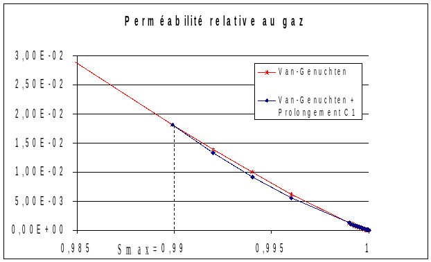
Figure 2.5.2-a : Example of extending relative permeability

For suction \(S(\mathit{Pc})\) and for \(\mathit{Pc}<\mathit{Pcmin}\) (with \(S(\mathit{Pcmin})=\mathit{Smax}\)) we extend the curve \(S(\mathit{Pc})\) by a hyperbola such that the curve is \(\mathit{C1}\) at this point:

For \(S>\mathit{Smax}\):

\(S(\mathit{Pc})=1{-}\frac{A}{B{-}{P}_{c}}\)

With \(A\) and \(B\) such that the curve is \(\mathit{C1}\) in \(\mathit{Smax}\).

So we do have a decreasing curve that tends to 1 when \(\mathit{Pc}\) tends to \({-}\mathrm{\infty }\). This treatment allows us to manage negative capillary pressures in Code_Aster (see example).

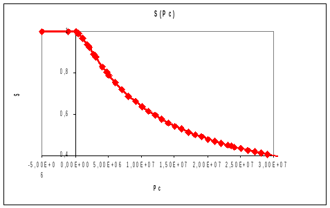
Figure 2.5.2-b : Example of an extension for PC<0

\(S(\mathit{Pc})\) is then multiplied by a « safety » coefficient \(\mathit{CSAT}\) so that saturation never reaches 1 (a problem that we don’t know how to deal with).

Tip: we recommend a value of \(\mathit{CSAT}\) as close as possible to \(1.\) ( \(\mathrm{0.99999}\) for example) .

Or he chooses HYDR_TABBAL which uses a poromechanical formulation valid for relative humidity ranges below 50% (model based on the thesis of Ginger El Tabbal [1]). In this case, the parameters corresponding to the saturation curve and its derivative as well as the relative permeabilities and their derivative are defined by the user in the same way as with HYDR_UTIL. In addition, all the parameters specific to the hydr_tabbal law:Math: t (mathit {HR}) `, :math: {A} _ {0} , :math: {S} _ {mathit {BJH}}} , :math: `t (mathit {BJH}}}, :math: {BJH}}, :math: {BJH}}, :math: {left}}, :math: {left}} (frac {partialgamma} {partial {epsilon} _ {s}}right) |} _ {mu} `should be defined in DEFI_MATERIAL:

\(t(\mathit{HR})\) corresponds to the parameter « EPAI »

\({A}_{0}\) corresponds to the A0 parameter

\({S}_{\mathit{BJH}}\) corresponds to the parameter « S_BJH »

\({\mathrm{\omega }}_{\mathit{BJH}}\) corresponds to the parameter « W_BJH »

math:

{left (frac {partialgamma} {partialgamma} {partial {epsilon} _ {s}}right) |} _ {mu} corresponds to the SHUTTLE parameter

A method for calculating these parameters is defined in the Appendix.

Attention:

Depending on the KIT_XXXX chosen, not all behaviors are legal (for example if you choose an unsaturated porous medium, you cannot affect an ideal gas-type behavior). all possible combinations are summarized below

	Mechanic	Hydraulic Coupling	Hydraulic Law
KIT_HM KIT_THM	“ELAS”, “MOHR_COULOMB”, “CJS”, “HUJEUX”, “LAIGLE”, “CAM_CLAY”, “DRUCK_PRAGER”, “LEK”, “DRUCK_PRAG_N_A”, “VISC_DRUCK_PRAG”, “GONF_ELAS”, “HOEK_BROWN_TOT”, “HOEK_BROWN_EFF”,	“GAZ”, “”, “LIQU_SATU”, “LIQU_GAZ_ATM”	“HYDR_UTIL”
KIT_HM KIT_THM	“MAZARS”, “ENDO_ISOT_BETON”,	“GAZ”, “LIQU_SATU”,
“LIQU_GAZ_ATM” »	“HYDR_ENDO”
KIT_HHM KIT_THHM	“ELAS”, “MOHR_COULOMB”, “CJS”, “HUJEUX “”LAIGLE”, “CAM_CLAY”, “DRUCK_PRAGER”, “DRUCK_PRAG_N_A”, “VISC_DRUCK_PRAG”, “GONF_ELAS”, “LEK”, “HOEK_BROWN_TOT”, “HOEK_BROWN_EFF”, “BARCELONE”	“LIQU_GAZ”, “LIQU_VAPE_GAZ”, “LIQU_AD_VAPE_GAZ” “LIQU_AD_GAZ”	“HYDR_UTIL” “HYDR_VGM” “HYDR_VGC” “HYDR_TABBAL”
KIT_HHM KIT_THHM	“MAZARS_UNIL”, “ENDO_ISOT_BETON”,	“LIQU_GAZ”, “LIQU_VAPE_GAZ”,
“LIQU_AD_VAPE_GAZ”
“LIQU_AD_GAZ” »	“HYDR_ENDO”
KIT_THH KIT_HH		“LIQU_GAZ”, “”, “LIQU_VAPE_GAZ”, “LIQU_AD_VAPE_GAZ” “LIQU_AD_GAZ”	“HYDR_UTIL” “HYDR_VGM” “HYDR_VGC” “HYDR_TABBAL”
KIT_THV		“LIQU_VAPE”	“HYDR_UTIL”

Note:

In case of convergence problems, it can be very useful to activate linear search. However, linear research does not systematically improve convergence, so it should be handled with care.

2.6. Post-treatment#

2.6.1. Generalities#

Data post-processing in THM does not vary from the usual Aster post-processing. Just remember that for any impression of the values at the nodes that are not the nodal unknowns, it is necessary to calculate these values using the « CALC_CHAMP » command, an example of which is given below.

For constraints:

U0= CALC_CHAMP (reuse =U0,

MODELE = MODELE,

CHAM_MATER = CHMAT0,

TOUT_ORDRE =” OUI “,

CONTRAINTE =( “SIGM_ELNO”),

RESULTAT =U0,);

For internal variables:

U0= CALC_CHAMP (reuse =U0,

MODELE = MODELE,

CHAM_MATER = CHMAT0,

TOUT_ORDRE =” OUI “,

VARI_INTERNE =( “VARI_ELNO”),

RESULTAT =U0,);

However, it should be remembered that all output displacement values correspond to \({u}^{\text{ddl}}\) and not \(u={u}^{\text{ddl}}+{u}^{\text{ref}}\).

It is also important to know the names of the constraints and the numbers of the internal variables. All of this is recorded in Appendix I.

Thus the following example makes it possible to print the mass of liquid water on the group of nodes \(\mathit{HAUT}\) at all times.

TAB1 = POST_RELEVE_T (ACTION =_F (INTITULE =” CONT “,

GROUP_NO =( “HAUT”),

RESULTAT =U0,

NOM_CHAM =” SIEF_ELNO “,

TOUT_ORDRE =” OUI “,

NOM_CMP =( “M11”),

OPERATION =” EXTRACTION “,),);

IMPR_TABLE (TABLE = TAB1,

FICHIER =” RESULTAT “,

FORMAT =” AGRAF “,

PAGINATION =” INST “,

NOM_PARA =( “INST”, “COOR_X”, “M11”),);

The following example allows you to print the porosity values at node 1 and at the first point in time.

TAB2 = POST_RELEVE_T (ACTION =_F (INTITULE =” DEPL “,

NOEUD =” NO1 “,

RESULTAT =U0,

NOM_CHAM =” VARI_ELNO “,

NUME_ORDRE =1,

NOM_CMP =( “V2”),

OPERATION =” EXTRACTION “,),);

IMPR_TABLE (TABLE = TAB2,

FICHIER =” RESULTAT “,

FORMAT =” AGRAF “,

PAGINATION =” INST “,

NOM_PARA =( “INST”, “COOR_X”, “V2”),);

2.6.2. Internal variables#

In addition to the generalities proposed above, there is now a more user-friendly way to extract internal variables (cf. [U4.81.01]). To do this, fields have been created whose principle is to extract from the field « VARI_ELGA » (or « VARI_ELNO » for fields calculated at the nodes) the internal variable that interests us via a keyword that is more meaningful than \(\mathit{V1}\), \(\mathit{V2}\),…

As post-processing these fields are calculated by « CALC_CHAMP ». The syntax to use is as follows:

for a field with cham_elem elements

GAMP = CALC_CHAMP (RESULTAT =U0,

OPTION =' VAEX_ELNO ',

NOM_VARI =' GAMP ');

for a field with cham_no nodes:

GAMP = CALC_CHAMP (reuse= GAMP,

RESULTAT = GAMP,

VARI_INTERNE =' VAEX_NOEU ');

Since it’s just a matter of extracting one (and only one!!) internal variable, the corresponding elem_fields must have been calculated beforehand:

U0= CALC_CHAMP (reuse =U0,

MODELE = MODELE,

CHAM_MATER = CHMAT0,

TOUT_ORDRE =” OUI “,

VARI_INTERNE =( “VARI_ELNO”),

RESULTAT =U0,);

The list of the various symbolic names for the internal variables is:

“DPORO”	variation in material porosity
“DRHOLQ”	variation in the density of the material
“DPVP”	change in vapour pressure
“SATLIQ”	liquid saturation
“EVP”	cumulative volume plastic deformation
“IND_ETA”	Mechanical status indicator
“D”	Damage value
“IND_END”	Damage indicator
“TEMP_MAX”	Maximum Temperature
“GAMP”	Cumulative plastic deviatory deformation
“PCR”	Critical Pressure
“SEUIL_HYD”	Water threshold
“IND_HYD”	Water Irreversibility Indicator
“PCOHE”	Cohesion pressure
“COMP_ROC”	Rock behavior
“SEUIL_ISO”	Isotropic threshold
“ANG_DEV”	Deviatory threshold angle
“X11”	Components of the kinematic work hardening tensor
“X22”	Components of the kinematic work hardening tensor
“X33”	Components of the kinematic work hardening tensor
“X12”	Components of the kinematic work hardening tensor
“X13”	Components of the kinematic work hardening tensor
“X23”	Components of the kinematic work hardening tensor
“DIST_DEV”	Normalized distance to the deviation threshold
“DEV_SUR_CRIT”	Relationship between the deviatory threshold and the critical deviatory threshold
“DIST_ISO”	Normalized distance to the isotropic threshold
“NB_ITER”	Number of internal iterations
“ARRET”	Value of the local test to stop the iterative process
“NB_REDE”	Local time step redistribution number
“SIGNE”	Sign of the contracted product of the deviatoric stress by the deviatoric plastic deformation

Note:

When the variable to be extracted is not part of the internal variables of the laws concerned, an alarm is issued but the field is still assigned to R 8VIDE () .

2.6.3. Isovalues#

Attention: distinction between linear resolution and quadratic meshing

It should be noted that for any problem THM and in order to avoid any ambiguity for the user, the mesh used is always quadratic. On the other hand, the resolution of the hydraulic and thermal problem is linear: the unknowns \(\mathit{PRE1}\), \(\mathit{PRE2}\) and \(\mathit{TEMP}\) therefore only exist on the top nodes of the mesh.

At the end of the calculation, we obtain a result in this form:

Pressures \(\mathit{PRE1}\), \(\mathit{PRE2}\) and temperatures \(\mathit{TEMP}\) are on the top nodes of the elements.
The internal variables, the constraints are on the gauss points and/or the nodes of the quadratic mesh (depending on whether we are selective or lumped) and the mechanical displacements are on the vertices and the middle nodes.

There is therefore a conflict between quadratic meshes and linear calculations, which will pose a problem, for example, when drawing isovalues.

There is then a simple way to get rid of this problem by projecting all the results onto the linear mesh resulting from the quadratic mesh. So all the results will be defined in the same place (on the summits).

For \(\mathit{TEMP}\), \(\mathit{PRE1}\) and \(\mathit{PRE2}\), simply project as shown in the following example:

## projection of the quadratic mesh onto the linear mesh:

MAILQ4 = CREA_MAILLAGE (

MAILLAGE = MAIL,

QUAD_LINE = _F (TOUT = “OUI”),

## assignment of the corresponding model:

MODELQ4 = AFFE_MODELE (MAILLAGE = MAILQ4,

AFFE =_F (TOUT =” OUI “,

PHENOMENE =” MECANIQUE “,

MODELISATION =” D_PLAN “,),);

## projection of the result on this new model:

RESULIN = PROJ_CHAMP (

METHODE =” ELEM “,

RESULTAT =resu,

MODELE_1 = MODELQ8,

MODELE_2 = MODELQ4,

NOM_CHAM =” DEPL “,

TOUT_ORDRE =” OUI “)

## usual post-processing but on the linear mesh:

IMPR_RESU (FORMAT =” MED “,

RESU =_F (

RESULTAT = RESULIN,

NUME_ORDRE =( 1,10,20,),

NOM_CMP = (“PRE1”, “PRE2”,),

MAILLAGE = MAILQ4,),);

There is an alternative method, which may prove to be faster for large industrial studies. This method uses « MACR_ADAP_MAIL » [U7.03.01]. It is assumed that resu is composed of nbinst moments stored in the linst list. The previous post-processing can also be done in the following manner:

PRE = [None] *nbinst;

PREB = [None] *nbinst;

for k in range (nbinst):

PRE [k] = CREA_CHAMP (TYPE_CHAM =” NOEU_DEPL_R “,

OPERATION =” EXTR “,

RESULTAT =resu,

NOM_CHAM =” DEPL “,

INST =linst [k],);

word1= {}

word2 = {}

word1 [“MAJ_CHAM”] = []

word2 [“AFFE”] = []

for k in range (nbinst):

PREB [k] =CO (”PREB_ %d”% (k))

word1 [“MAJ_CHAM”] .append (

_F (TYPE_CHAM =” NOEU_DEPL_R “, CHAM_GD = PRE [k],

CHAM_MAJ = PREB [k],),);

word2 [“AFFE”] .append (

_F (CHAM_GD = PREB [k], INST =linst [k],),);

MACR_ADAP_MAIL (ADAPTATION =” MODIFICATION “, DEGRE =” OUI”,

MAILLAGE_N = MAILQ8,

MAILLAGE_NP1 = CO (“MAILQ4”),

word 1);

RESULINB = CREA_RESU (OPERATION =” AFFE “, TYPE_RESU =” EVOL_NOLI”, NOM_CHAM =” DEPL “, **word2);

2.7. Some test cases#

For information, we summarize here some test cases available in the Code_Aster database. This list is by no means exhaustive but provides direct access to a number of representative examples.

Test case name	Modeling type THM	Represented phenomenon	Geometric modeling	Coupling law
wtna109A	AXIS_THVD	Desaturation by heating of an airless medium	axisymmetric	LIQU_VAPE
wtna110a	AXIS_HH2MS	Modeling a swelling of a clay	axisymmetric	LIQU_AD_GAZ_VAPE
Wtna107	AXIS_THMS	Heating a saturated medium (THM)	axisymmetric	LIQU_SATU
wtna112	AXIS_THMS	Thermal pressurization of a drained specimen	axisymmetric	LIQU_SATU
wtnP117a	D_PLAN_HHS	Capillary rebalancing of 2 materials (BO/BG)	plane	LIQU_GAZ
wtnP118a	D_PLAN_HH2D	Column gravity rebalancing	plane	LIQU_AD_GAZ_VAPE
wtnP112d	D_PLAN_HMD	Restoring a column (Richards” hypothesis)	plane	LIQU_GAZ_ATM
wtnp101a	D_PLAN_HM	Modeling a gas-saturated medium	plane	GAZ
wtnl100A	D_PLAN_HMD D_PLAN_HM_SI	Consolidation problem (Therzagi)	plane	LIQU_SATU
wtnv123A	3D_HHM	Hydrostatic then triaxial test with fixed suction (Barcelona model)	3D	LIQU_GAZ
wtnP113a	D_PLAN_THHD	Restoration of a cell by the massif	plane	LIQU_GAZ
wtnv121a	3D_HHMD	Concrete wetting with damage	3D	LIQU_GAZ
wtnV130a	3D_THH2S	Heating a porous medium with dissolved air	3D	LIQU_AD_GAZ_VAPE
wtnv140	3D_HMS	Anisotropic Drained Triaxial Test	3D	LIQU_SATU