4. Anisothermal simulations#
During anisothermal simulations, the variation of parameters with temperature must most of the time be taken into account. It is therefore necessary to ensure the correct identification of these parameters.
In this paragraph, some classical errors induced by the interpolation or extrapolation of values as a function of temperature are illustrated.
The tests are carried out with laws VMIS_ISOT_TRAC and VMIS_CIN1_CHAB. However, the conclusions reached are not exclusive to a particular law.
4.1. Dangers of extrapolation:#
To conduct a thermo-mechanical study with a law of behavior whose coefficients depend on temperature, the user may want to extrapolate his curves to carry out his study at a given temperature. This is strongly discouraged. An example:
In the case of isotropic work hardening, it is common to use experimental traction curves for a few temperatures, varying for example between \(20°\) and \(350°\). The traction curves are entered in the command file for various temperatures with the command “DEFI_NAPPE “.Assume that we have defined the extensions by PROL_DROITE =” LINEAIRE” and PROL_GAUCHE =” LINEAIRE “and =””.
It is assumed that the user wishes to perform a calculation at a temperature that exceeds the maximum temperature at which the identifications of the traction curves were made, i.e. 1000° C. for example (this is a deliberately exaggerated example, but which illustrates the point). The material coefficients of the law would therefore be obtained at \(1000°C\) by extrapolation.
This can lead to aberrant results (Figure 4.1-a): the traction curve obtained at the extrapolated temperature of \(1000°C\) has a concavity and a collaring slope that is contradictory to the other curves and to reality.
To avoid this type of error, any extrapolation with respect to temperature should be avoided.

Figure 4.1-a *. Tensile curves as a function of temperature — result at* \(1000°C\)
4.2. Error in temperature interpolation#
This example highlights a possibility of error in temperature interpolation, generally due to a non-monotonic evolution of material coefficients with temperature. It is sufficient that only one of the coefficients does not evolve monotonically for the interpolation between two traction curves to lead to a curve that is not between the two extremes.
To show this kind of error, with a typical law of behavior “VMIS_CIN1_CHAB”, we set up the following test:
Assume three known traction curves identified experimentally at 3 different temperatures: \(20°\), \(100°\) and \(200°C\). We are trying to identify the parameters of the “VMIS_CIN1_CHAB” law at these three temperatures. To fully understand, let’s briefly recall the form of collaring in the “VMIS_CIN1_CHAB” law:
Criteria: \({(\sigma \mathrm{-}C\alpha )}_{\text{eq}}\mathrm{-}R(p)\mathrm{\le }0\)
kinematic work hardening: \(\dot{\alpha }\mathrm{=}\dot{{\varepsilon }^{p}}\mathrm{-}\gamma \alpha \dot{p}\)
isotropic work hardening: \(R(p)\mathrm{=}{R}_{\mathrm{\infty }}+({R}_{0}\mathrm{-}{R}_{\mathrm{\infty }}){e}^{\mathrm{-}\text{bp}}\)
Suppose that the results of 3 identifications at three different temperatures are:
to \(T\mathrm{=}20°\); the identified material parameters are: \({C}_{1}\), \({\gamma }_{1}\), \({R}_{0}\), not zero, and \({R}_{\mathrm{\infty }}\mathrm{\simeq }{R}_{0}\) \(b\mathrm{\simeq }0\), (i.e. an almost pure kinematic behavior);
to \(T\mathrm{=}100°\); the identified material coefficients are: \({C}_{2}\mathrm{\simeq }0\), \({R}_{0}\), \({R}_{\mathrm{\infty }}\), \({b}_{2}\). non-zero, (i.e. an almost pure isotropic behavior)
to \(T\mathrm{=}200°\); the material coefficients are: \({C}_{3}\), \({\gamma }_{3}\), \({R}_{0}\),, non-zero, \({R}_{\mathrm{\infty }}\mathrm{\simeq }{R}_{0}\), \({b}_{3}\mathrm{\simeq }0\), (again pure kinematic behavior).
Each of these identifications is sufficiently precise, and makes it possible to find, for each temperature, numerical curves that are very similar to the experimental curves.
The simulation of the traction curve at the temperature of \(50°C\) is shown in the figure)
It can be seen that the curve obtained by interpolation at \(50°C\) is erroneous:
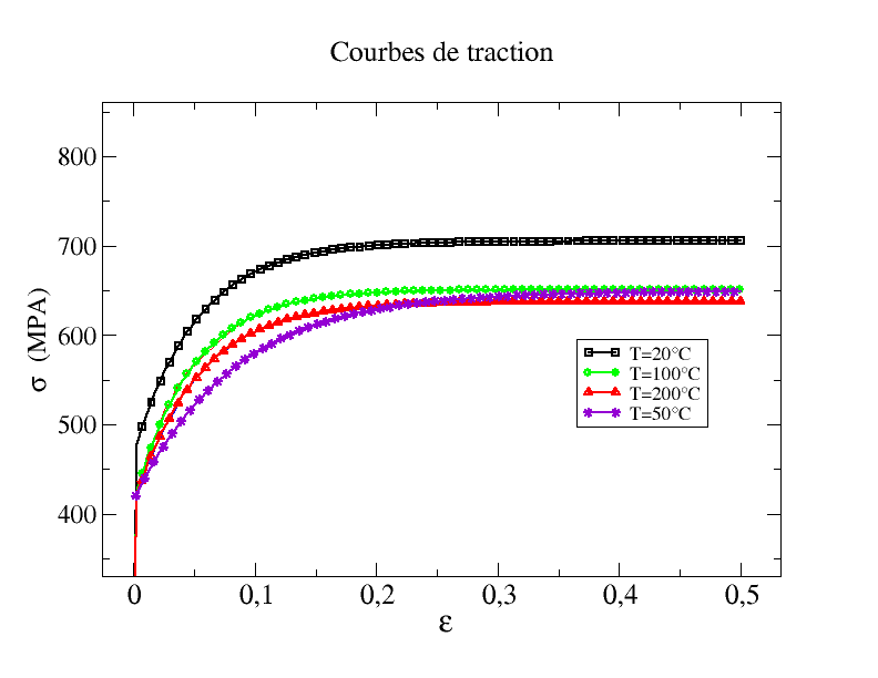
Figure 4.2-a *. Tensile curves as a function of temperature — result at 50°*
This is due to the fact that the identifications were made independently, without verifying the consistency of the results. The variations of each coefficient with temperature are enormous: for example
Temperature °C |
\(C\) |
|
\(20\) |
|
|
\(\mathrm{\simeq }0\) |
|
|
\({C}_{3}\) |
|
This example is of course extreme, but it makes it possible to make a recommendation:
either check the monotonic evolution of the material parameters as a function of temperature, and repeat the identification for suspicious values,
or, if possible, carry out the identification at once for all temperatures.