2. Loads, boundary conditions, initial conditions#
2.1. Core of the problem#
Loads and boundary conditions are important for good modeling. Their influence on the results is most of the time direct, so that their application can be verified by a simple preliminary calculation, for example using MECA_STATIQUE, or by visualizing the boundary conditions via the CONCEPT keyword from IMPR_RESU in format MED.
As far as boundary conditions are concerned, it is often a question of introducing the minimum of them to block the movements of rigid solid, therefore to avoid having floating bodies in the structure, which would cause a zero pivot or a singular matrix during the resolution.
Some boundary conditions are non-linear, for example one-sided contact. Their verification cannot therefore be done using a first linear calculation (MECA_STATIQUE): the various objects in contact must not have rigid body movements u2.04.04. If this is the case, zero pivots can be avoided by adding discrete elements (springs) of low rigidity.
Loads (other than blockages) can consist either of imposed travel conditions, or of imposed efforts, or of an imposed initial field type.
In all cases, it is important to represent reality well. Symmetry or antisymmetry conditions can be used to advantage [1].
In general, an imposed displacement condition does not provide the same results as an imposed force condition: a displacement imposed on a part of the border requires that the (imposed) displacement be constant in space on this part, therefore brings rigidity, or even singularities. Take the example of the punching of a massif: the displacement imposed on the edge of the punch induces stress singularities of the same nature as those encountered at the bottom of a crack.
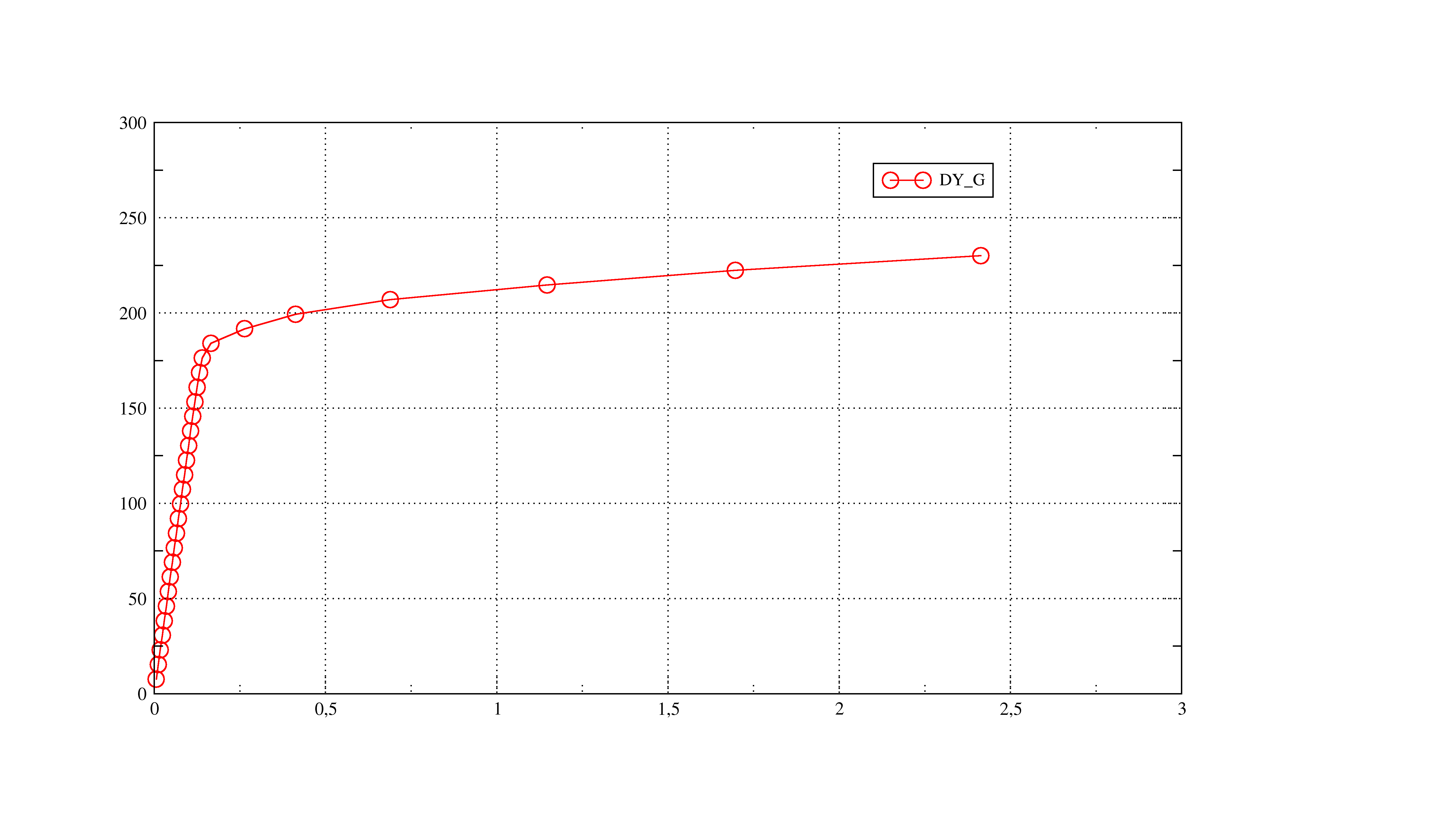
Figure 2.1-1: Example of a force-displacement curve
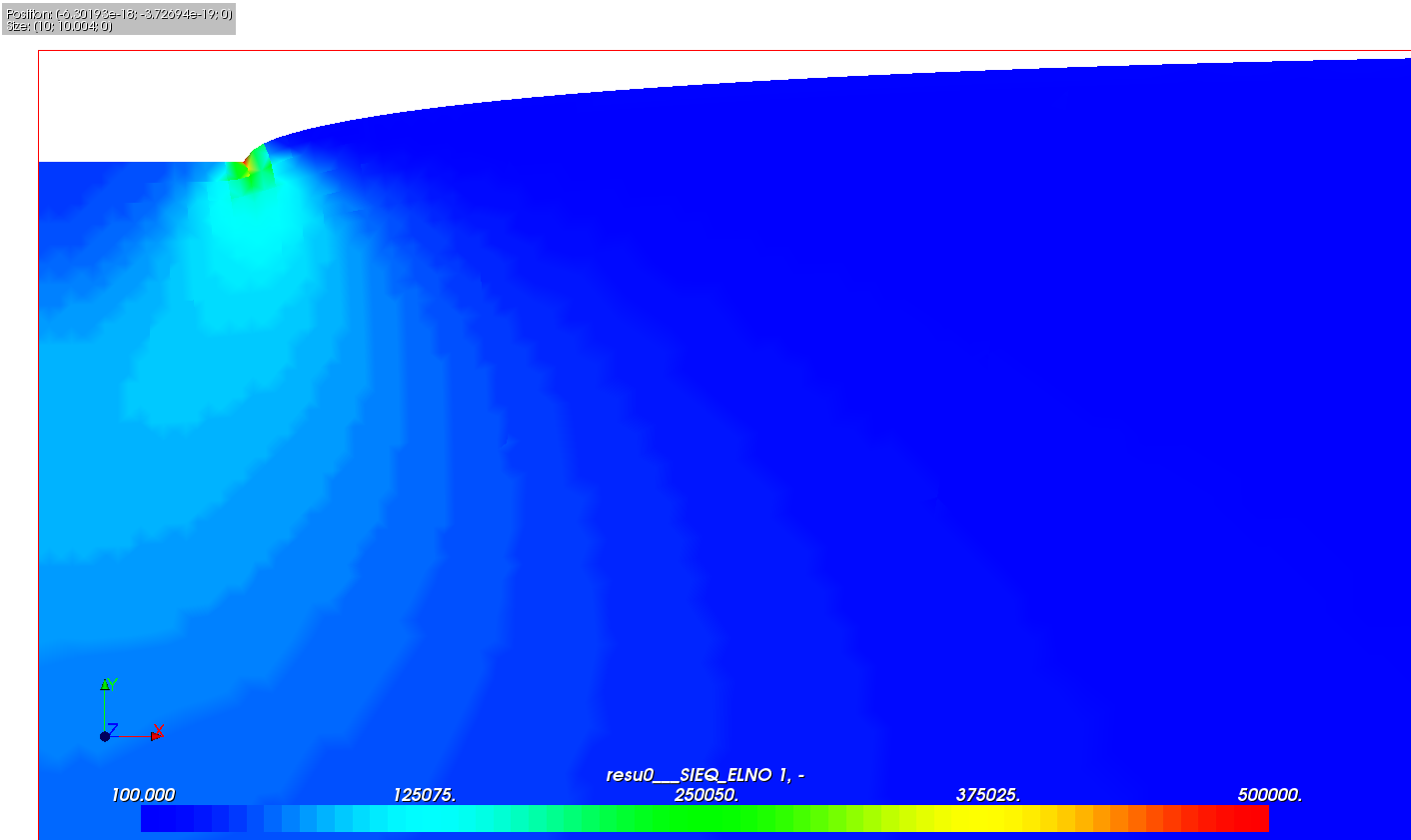
Figure 2.1-2: punching with imposed displacement
Moreover, for non-linear calculations, the conduct of the calculation is not the same: in case of softening or limiting load, loading with imposed force may be unlawful (beyond the limit load). Take for example punching (see and): the response in terms of the resultant force on the punch as a function of the displacement shows that the more the imposed force approaches the limit load, the more difficult the convergence will be, until it is impossible beyond the limit load. If the correct modeling requires applying an imposed force, the problem can be solved via by controlling the imposed force in relation to the movement of a point or a set of points (continuation or arc-length method) (see r5.03.80 r5.03.80).
The user documentation relating to the application of loads and boundary conditions are u4.44.01 u4.44.01 u4.44.01 and u4.44.03 u4.44.03 u4.44.03.
2.2. Precautions for applying loads#
It is useful for the loading application to browse the various keywords of u4.44.01 u4.44.01. Attention to the vocabulary, in particular, loads of the type FORCE_FACE, PRES_REP,, FORCE_CONTOUR,,, FORCE_ARETE,, FORCE_INTERNE,, FORCE_COQUE, FORCE_TUYAU correspond to distributed forces (linear, surface, volume) and are expressed in stress unit (for example \(\mathit{Pa}\) in S.I. units). Only FORCE_NODALE are expressed in units of forces (\(N\)), and the distributed forces of beams (FORCE_POUTRE) in units of force divided by a length.
With regard to pressures (PRES_REP, FORCE_COQUE/PRES), the pressure applied is positive in the opposite direction from normal to the element. It is strongly recommended to reorient these normals via the MODI_MAILLAGE operator, keywords ORIE_PEAU_ *, ORIE_NORM_COQUE.
For 2D, 3D continuous environments, the use of point forces (FORCE_NODALE) should be avoided, as it always leads to singularities.
The application of time-dependent loads can be done in two ways:
either by defining constant loads, then by applying a multiplying factor as a function of time to these loads during the resolution (keyword FONC_MULT under EXCIT in STAT_NON_LINE),
or by directly defining time-dependent loads via AFFE_CHAR_MECA_F.
In the case where the loads are of the imposed displacement type, they can be introduced either by AFFE_CHAR_MECA (_F), or by AFFE_CHAR_CINE (_F). The use of this last one command saves calculation time, which can be appreciable in a non-linear way (because it does not add Lagrange multipliers, so there are fewer equations to solve).
Command variables are not part of AFFE_CHAR_MECA (_F) commands. However, in many models, they can be assimilated to loads: for example, thermal expansion can by itself generate states of stresses and deformations leading to non-linearities in behavior. Command variables are applied via AFFE_MATERIAU.
However, it is necessary to note here a modeling precaution concerning these control variables: in fact, as soon as the calculation is incremental, STAT_NON_LINE uses the control variable increment at each time step to calculate the corresponding deformations (see for example r5.03.02 Integration of Von Mises elasto-plastic behavior relationships). In general, it is preferable that, at the initial moment, the structure be unstressed, not deformed. If this is not the case, you must add a preliminary moment when the structure is at rest, see for example test FORMA30 v7.20.101 FORMA30 - Thermoelastic hollow cylinder. In case of detection of constraints due to the control variables at the initial moment, the alarm is obtained:
<A><MECANONLINE2_97>:
-> The initial command variables induce incompatible constraints:
the initial state (before the first moment of calculation) is such that the control variables (temperature, hydration, drying, etc.) lead to unbalanced constraints.
-> Risk & Advice: in the case of an incremental resolution, we only consider the variation of the control variables between the previous moment and the current moment. Therefore, any incompatible constraints due to these initial control variables due to these initial control variables are not taken into account.
To take these constraints into account, you can:
Starting from an earlier fictitious moment when all control variables are zero or equal to the reference values
choose appropriate reference values
For more information, see the documentation for STAT_NON_LINE (U4.51.03) keyword EXCIT, and the FORMA30 test (V7.20.101).
2.3. The different types of boundary conditions#
The simplest boundary conditions serve primarily to introduce symmetry conditions, on the one hand, and to prevent rigid solid movements, on the other hand. When they are of the imposed degree of freedom type, we can use either AFFE_CHAR_MECA, or (to optimize the calculation time) AFFE_CHAR_CINE u2.01.02.
Methodological advice: it is always better to apply boundary conditions to groups of meshes rather than to groups of nodes or lists of nodes or meshes. In fact, the groups of cells correspond to geometric areas, and are retained during a refinement of the mesh (manual or using Lobster), while the groups of nodes are modified. This is why in AFFE_CHAR_MECA the keywords DDL_IMPO, FACE_IMPO, LIAISON_UNIF, as well as all the keywords in AFFE_CHAR_CINE include the keyword GROUP_MA, which should therefore be preferred.
It is sometimes necessary to impose linear relationships between degrees of freedom. The LIAISON_ * keywords in AFFE_CHAR_MECA allow this type of relationship to be introduced. Elementary relationships can be defined using LIAISON_DDL, but it becomes tedious if there are a lot of equations to write. Higher-level features are available, for example:
- LIAISON_SOLIDE to rigidify part of the structure, (in small deformations and small movements only)
- LIAISON_UNIF to ensure that part of the border will keep the same movement (unknown at first glance);
u4.44.01 u4.44.01
LIAISON_MAIL, LIAISON_GROUP to connect two edges,
and other AFFE_CHAR_MECA specific keywords.
In addition, it is possible to connect (in the energetic sense) models of different types, via LIAISON_ELEM and several options (in small deformations and small displacements only)
“COQ_TUYAU”, “3D_ TUYAU “, pipe elements with with plates and shells, 3D;
- “COQ_POU”, beams or discrete ones with plates and shells
Note: in some cases, boundary conditions or imposed displacement-type loads are not suitable because they provide too much local rigidity. It may be interesting to replace these conditions by a connection between the part of the border concerned and a discrete element, on which the imposed travel conditions or a twister of imposed forces will be applied. This means that the movements of the border will be equal on average to the displacement of the discrete element, without introducing parasitic constraints. On the other hand, this method introduces additional degrees of freedom (Lagrange multipliers), so the resolution of linear systems can be more expensive.
Unilateral contact, with or without friction, is a particular type of boundary conditions. It is highly non-linear, and its processing in STAT_NON_LINE/DYNA_NON_LINE requires additional iterations to achieve convergence. It is strongly recommended to consult the document u2.04.04 u2.04.04 u2.04.04 to model these phenomena correctly.
2.4. The initial conditions#
In AFFE_CHAR_MECA, it is possible to define average strain loads or average stress loads that are globally uniform (keywords PRE_EPSI, PRE_SIGM).
These loads should not be confused with the initial deformations and stresses used in nonlinear mode, because these quantities do not intervene directly in the expression of the law of behavior, but only on the second limb.
The initial fields of constraints, displacements and internal variables are to be provided directly in STAT_NON_LINE (keyword ETAT_INIT). To build these fields, it may be useful to consult the document u2.01.09.