3. Case creation

Start the MasterStudy module.

3.1. Thermal calculation

Add a stage by clicking on the « Addstage » button on the toolbar.

• A Stage_1 step is added in Data Settings.

Rename the step to « Thermal_Calculation », by selecting the step and then typing F2 or using the « Rename » context menu.

Order LIRE_MAILLAGE

On the toolbar, in the « Mesh » drop-down list, select the « Read a mesh » command.

• The « Mesh » folder with a « mesh » command is added to the step.

• The editing panel opens on the right.

In the « Mesh file location » field (UNITE), click on the « … » selection button and select the « lot6.mmed » mesh file.

Change the name of the order in the « Name » field to « MAIL ».

Then, check the « Mesh file format » box (FORMAT).

Then, select the « Med » option from the dropdown list.

Validate by clicking on the « OK » button.

• The edit panel disappears and the command is renamed.

Order MODI_MAILLAGE

Add a MODI_MAILLAGE command by clicking on the « Show All Commands » button in the toolbar, the search panel appears on the right.

Type MODI_MAILLAGE in the search field.

Then double click on item MODI_MAILLAGE.

• A mesh0 command is added to the step.

• The editing panel opens on the right.

Select « MAIL (LIRE_MAILLAGE) » as the value for the « Mesh » field.

Check the « ORIE_PEAU » box.

Click on the « Add an occurrence » button, then on the « Edit » button, then « Edit » in the Group of element field (GROUP_MA_PEAU). In the « Manual selection » field, enter « SURFINT » or check the « SURFINT » box and click on the « OK » button.

Validate by clicking on the « OK » button on each panel (2 times).

• The panel closes.

Order DEFI_MATERIAU

Add the DEFI_MATERIAU command, either using the search or directly in the « Material/Define a material » toolbar.

• A « subdue » command and the « Material » folder are added to the step.

• The editing panel opens on the right.

Rename the command « MATER » and enter the following values:

• Check the « Linear isotropic elasticy » box (ELAS) then click on the « Edit » button.

  • Young’s modulus (E) = 204000000000.

  • Fish’s ratio (NU) = 0.3.

  • Check the « Thermal expansion coefficient » box (ALPHA) = 1.096e-05.

  • Click on the « OK » button.

• Use the search field to find field THER then check the « Isotropic heat conduction » box (THER).

  • Click on the « Edit » button.

  • Thermal conductivity (LAMBDA) = 54.6.

  • Check the « Volumetric heat capacity » box (RHO_CP) = 3710000.

  • Click on the « OK » button.

• Confirm the order by clicking on the « OK » button.

• The panel closes.

Order AFFE_MODELE

Add a AFFE_MODELE command, either using the search or directly in the « Model Definition/Assign finite element » toolbar. And fill in the fields:

• Name = MODTH

• Mesh = MAIL (MODI_MAILLAGE)

• Check the « Finite element assignment » box (AFFE), then add an element by clicking on the « Add an occurrence » button, then « Edit ».

  • Check the « Everywhere » box (TOUT) and select « Yes. »

  • Phenomenon (PHENOMENE) = Thermic (THERMIQUE).

  • Modeling (MODELISATION) = 3D.

  • Click on the « OK » button.

• Confirm the order by clicking on the « OK » button.

• The panel closes.

Order AFFE_MATERIAU

Add a AFFE_MATERIAU command, either using the search or directly in the « Material/Assign a material » toolbar. And fill in the fields:

• Name = CHMATER.

• Check the « Mesh » box = MAIL (MODI_MAILLAGE).

• For the « Material assignment » field (AFFE), click on the « Add an occurrence » button, then « Edit ».

  • Check the « Everywhere » box (TOUT) and select « Yes. »

  • Material (MATER), click on the « Add an occurrence » button and select « MATER ».

  • Click on the « OK » button.

• Confirm the order by clicking on the « OK » button.

• The panel closes.

Order DEFI_FONCTION

Add a DEFI_FONCTION command, either using the search or directly in the « Functions and Lists/Define function » toolbar. And fill in the fields:

• Name = F_ TEMP.

• Parameter name (NOM_PARA) = Time (INST).

• Check the « Coordinates » box (VALE), click on the « Edit » button and enter the lines (0, 20) then (10, 70), then validate with OK.

• Confirm the order by clicking on the « OK » button.

Order AFFE_CHAR_THER_F

Add a AFFE_CHAR_THER_F command, either using the search or directly in the « BC and load/Assign variable thermal load » toolbar. And fill in the fields:

• Name = CHARTH.

• Model (MODELE) = MODTH.

• Check the « Enforce Temperature » box (TEMP_IMPO), click on the « Add an occurrence » button and then on « Edit ».

  • Check the « Group of element » box (GROUP_MA), click on the « Edit » button, then enter « SURFINT » in the manual field or check the « SURFINT » box and validate with OK.

  • Check the « Temperature » box (TEMP) = F_ TEMP.

  • Click on the « OK » button.

• Confirm the order by clicking on the « OK » button.

Order DEFI_LIST_REEL

Add a DEFI_LIST_REEL command, either using the search or directly in the « Functions and Lists/define a list of reals » toolbar. And fill in the fields:

• Name = LINST

• Check the « Value » box (VALE), click on the « Edit » button then enter the values 0, 5, 10.

• Click on the « OK » button.

• Confirm the order by clicking on the « OK » button.

Order DEFI_FONCTION

Add a DEFI_FONCTION command, either using the search or directly in the « Functions and Lists/Define function » toolbar. And fill in the fields:

• Name = F_ MULT.

• Parameter name (NOM_PARA) = Time (INST).

• Check the « Coordinates » box (VALE), click on the « Edit » button and enter the lines (0, 1) then (10, 1) and validate with OK.

• Confirm the order by clicking on the « OK » button.

Order THER_LINEAIRE

Add a THER_LINEAIRE command, either using the search or directly in the « Analysis/Linear thermal analysis » toolbar. And fill in the fields:

• Name = TEMPE.

• Model (MODELE) = MODTH.

• Material field (CHAM_MATER) = CHMATER.

• Loads (EXCIT), click on the « Add an occurrence » button then « Edit ».

  • Load (CHARGE) = CHARTH.

  • Check the « Multiply function » box (FONC_MULT) = F_ MULT.

  • Click on the « OK » button.

• For the « Initial condition » field (ETAT_INIT), click on the « Edit » button.

  • Check the « Value » box (VALE) = 20.

• Click on the « OK » button.

• For the « Timestepping » field (INCREMENT), click on the « Edit » button.

  • Time step list (LIST_INST) = LINST.

  • Click on the « OK » button.

• Confirm the order by clicking on the « OK » button.

Order IMPR_RESU

Add a IMPR_RESU command, either using the search or directly in the « Output/Set output results » toolbar. And fill in the fields:

• In the « Result file location » field (UNITE), click on the « … » selection button and choose the name and location of the output file in rmed format.

• Check the « Format » box = Med.

• For the « Results » field (RESU), click on the « Add an occurrence » button, then « Edit ».

  • Check the « Result » box (RESULTAT) = TEMPE.

  • Click on the « OK » button.

• Confirm the order by clicking on the « OK » button.

• Orders are created in step.

• A file is present in the « Data Files » tab.

Save the study by clicking on the « Save document » icon.

In the « Data Settings » tab, select the « Thermal Calculation » step, then « Export Command File » in the context menu. You can change the name of the command file or keep the name by default. Validate.

• The command file is generated.

• Verify that its content corresponds to the reference file.

3.2. Mechanical calculation

On the toolbar, click on the « Add stage from file » button.

Select the « lot6_stage2.comm » file.

• The step is imported in graphical mode.

Rename the step to « Calcul_Mecanique ».

3.3. Start the calculation

Go to the « History » view by clicking on the « History View » tab.

Click on the second step button (green cross).

• Both steps are automatically selected.

Click on the « Run » button to start the calculation.

• • A warning message indicates that the study should be saved prior to execution if the study has not been saved previously.

  Click on the « OK » button and save the study.

Click on the « Run » button again.

Note: it is important that both steps are successfully completed (green circle). If necessary, restart the calculation to obtain the expected result.

3.4. Post-treatment

Go to the « Case » view by clicking on the « Case View » tab.

Add a new stage by clicking on the « Addstage » button.

Put the step in text mode by selecting it and then choosing « Text Mode » from the context menu.

Rename the stage to Post_Processing.

Edit the step (double click).

• The text editor opens.

Copy the content of the « lot6_stage3.comm » file and add « UNITE =81 » to the « lot6_stage3.comm » file in the « IMPR_RESU » command:

then validate.

In the « Data Files » tab, click on « Post_Processing ».

Click on the « Add file » button in the Data Files panel.

In the « Mode » field, select « out ».

In the « Filename » field, click on the « … » selection button and choose the name and location of the output file in rmed format.

In the « Unit » field, enter 81.

Repeat the same procedure to add a file in tab format and unit = 8.

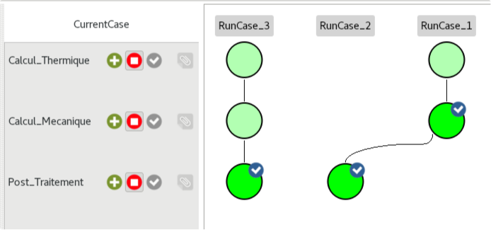
3.5. New execution

Go back to the « History View » tab.

• All three steps are visible.

Select « CurrentCase » to run the calculations.

Select the « Post_Treatment » step by clicking on the button (green cross).

• The previous steps are automatically selected to reuse the previous results (blue arrow).

Start the calculation.

• Only the last step is completed.

Select « CurrentCase ».

Select the first step again by clicking on the button (green cross).

• The first two steps are automatically selected to be re-executed (green cross).

Start the calculation.

• All three steps are completed.