3. Calculation steps#
3.1. Establishing the monotonic traction curve according to Ramberg Osgood#
In order to determine the reduction coefficients from spring factors (see § 3.5), a plastic behavior law according to Ramberg-Osgood is used.
The Ramberg-Osgood law is characterized by two parameters \(K\) and \(n\). The deformation is then written as a function of the stress:
\({ϵ=\frac{\sigma }{E}+ϵ}_{M,p}(\sigma )\)
where \(E\) is the Young’s modulus and \({ϵ}_{M,p}\) is the plastic deformation of the mean monotonic traction curve, defined by the power law:
\({ϵ}_{M,p}=K{(\frac{\sigma }{E})}^{1/n}\)
The material parameters of this law are given using the keyword POST_ROCHE (or POST_ROCHE_FO) from DEFI_MATERIAU. \(K\) corresponds to the RAMB_OSGO_FACT operand and \(n\) to RAMB_OSGO_EXPO.
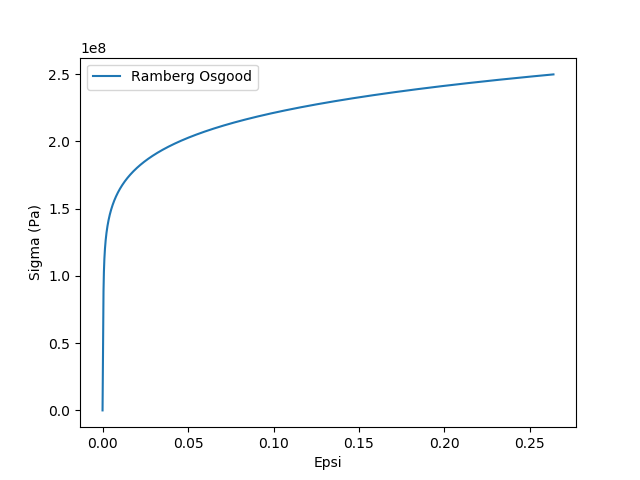
Image3.1-1 Example of Ramberg Osgood law.
3.2. Retrieving and classifying moments#
The moments are classified according to the curvilinear abscissa, for each section.
3.2.1. Ranking of moments according to CSM2#
The force-dependent moments (RB 3623.3) are due to:
by weight;
to the earthquake, quasi-static inertial part, if the 2nd method of ranking seismic moments CMS2 is applied; They are noted \({M}_{\mathit{SI}}\).
to the mechanical stresses applied (including pressure).
The moments dependent on travel (RB 3623.4) are due to:
to thermal expansion,
to the movements imposed on the anchorages; they are noted \({m}_{S}\).
to the earthquake, inertial part complements the quasi-static part, if the 2nd method for ranking seismic moments CMS2 is applied. They are rated \({m}_{\mathit{SI}}\).
3.2.2. Combination of moments according to CMS2 (RB 3645.82)#
Moments \({M}_{\mathit{SI}}\) are combined with the other « force-dependent » moments by adding the absolute values and assigning to each component the sign of the moment component due to permanent mechanical loads. The result is rated \(M\).
The \({m}_{S}\) moments are combined with the other « displacement-dependent » moments by giving them, for each component, the sign of the latter. The result is rated \(m\).
3.3. Calculation of reference stresses#
The reference stress is calculated for each section.
3.3.1. Reference stresses due to imposed displacements and thermal expansions#
The reference stress is calculated in accordance with §RB 3643.31 (Combination according to the 2nd method for classifying moments dependent on movements CMS2):
\({\sigma }_{\mathit{ref}}^{2}={\left(0.79{B}_{2}\frac{{m}_{R}^{\text{'}}}{Z}\right)}^{2}+{\left(0.87\frac{{m}_{1}}{Z}\right)}^{2}\),
where:
\({m}_{R}^{\text{'}}=\sqrt{{m}_{2}^{2}+{m}_{3}^{2}}\) is the resulting bending moment due to imposed displacements and thermal expansions (RB 3623.4),
\({m}_{1}\) is the torsional moment due to the imposed displacements (RB 3623.4),
\({B}_{2}=1\) stress coefficient (RB 3680) for straight sections (straight pipes, reducers, tee and sockets),
\({B}_{2}=\mathit{max}(\frac{1.30}{{f}^{2/3}},1.0)\) stress coefficient (RB 3680) for elbows and hangers,
\(f={h}_{c}\frac{{R}_{c}}{{r}_{m}^{2}}\) where \({r}_{m}=\frac{{D}_{e}-{h}_{c}}{2}\),
\({R}_{c}\) is the radius of curvature,
\({D}_{e}\) and \({h}_{c}\) correspond respectively to the outside diameter and to the thickness of the pipe,
\(Z\) is the moment of inertia, which is written for circular beams \(Z=\frac{{I}_{y}}{R}\), for the reductions we take the minimum of the ratio on the pipe element \(Z=\mathit{min}\frac{{I}_{y}}{R}\).
3.3.2. Inertial seismic reference constraints#
The reference stress is calculated in accordance with §RB 3643.31 (Combination according to the 2nd Seismic Moment Classification Method CMS2):
\({\sigma }_{S2,\mathit{ref}}^{2}={\left(0.79{B}_{2}\frac{{({M}_{S2})}_{R}^{\text{'}}}{Z}\right)}^{2}+{\left(0.87\frac{{M}_{S21}}{Z}\right)}^{2}\),
where:
\({({M}_{S2})}_{R}^{\text{'}}\) is the resulting inertial seismic bending moment (RB 3645.7 and RB 3645.82),
\({M}_{S21}\) is the inertial seismic torsional moment (RB 3645.7 and RB 3645.82),
the index \(S2\) relates to the combination CMS2,
\({B}_{2}\) is defined as in § 3.3.1.
3.4. Calculating reversibility#
The local reversibility is calculated for each section and the total reversibility for each line section.
3.4.1. Local reversibilities \(t\) and \({t}_{S}\)#
Local reversibility is defined by the elastic deformation to plastic deformation ratio, corresponding to the reference stress.
In each right section, the local reversibility linked to the reference constraints due to the imposed displacements is written:
\(\frac{1}{t}=\frac{{\epsilon }_{M,p}({\sigma }_{\mathit{ref}})}{\frac{{\sigma }_{\mathit{ref}}}{E}}\).
The local reversibility linked to seismic reference constraints is written as:
:math:`` \(\frac{1}{{t}_{S}}=\frac{{ϵ}_{M,p}({\sigma }_{S2,\mathit{ref}})}{\frac{{\sigma }_{S2,\mathit{ref}}}{E}}\).
3.4.2. Total reversibilities \(T\) and \({T}_{S}\)#
The total reversibility is calculated for each section of the pipe system with two fixed points.
The total reversibility linked to the reference constraints due to the imposed displacements is written as:
\(\frac{1}{T}\underset{0}{\overset{l}{\int }}{\sigma }_{\mathit{ref}}^{2}\mathit{Ads}=\underset{0}{\overset{l}{\int }}\frac{1}{t}{\sigma }_{\mathit{ref}}^{2}\mathit{Ads}\),
and the total reversibility linked to the seismic reference constraints is written as:
:math:`` \(\frac{1}{{T}_{S}}\underset{0}{\overset{l}{\int }}{\sigma }_{S\mathrm{2,}\mathit{ref}}^{2}\mathit{Ads}=\underset{0}{\overset{l}{\int }}\frac{1}{{t}_{S}}{\sigma }_{S\mathrm{2,}\mathit{ref}}^{2}\mathit{Ads}\),
where:
\(l\) is the length of the section of the curvilinear abscissa,
\(A\) is the area of the straight section along the curvilinear abscissa.
3.5. Calculating spring effect factors \({r}_{M}\) and \({r}_{S}\)#
The spring effect factor is calculated for each section, the maximums are calculated for each section.
3.5.1. Monotonous spring effect factor \({r}_{M}\)#
The monotonic spring effect factor \({r}_{M}\) quantifies the monotonic spring effect. It is calculated on each smallest part of the pipe system that has two fixed points.
This factor characterizes the difference between the stresses and deformations \({\sigma }_{\mathit{el}}\) and \({ϵ}_{\mathit{el}}\) calculated by assuming elastic behavior and the true values \(\sigma\) and \(ϵ\), linked by the monotonic tensile curve:
\({r}_{M}=-E\frac{ϵ-{ϵ}_{\mathit{el}}}{\sigma -{\sigma }_{\mathit{el}}}\)
This factor \({r}_{M}\) is:
zero when the spring effect is zero and the stress is purely secondary (the deformation is that calculated elastically)
infinity when the stress is purely primary (the stress is the one calculated elastically)
There is a \({r}_{M}\) factor in every pipe straight section:
\({r}_{M}=\mathit{max}(\frac{T}{t}-1;0)\)
3.5.2. Seismic spring effect factor \({r}_{s}\)#
Seismic spring effect factor \({r}_{s}\) quantifies the seismic spring effect:
\({r}_{s}=\frac{{T}_{s}}{{t}_{s}}-1\)
3.6. Calculation of the reduction coefficients \(g\) and \({g}_{S}\), for each section (case RCCM_RX =” NON “)#
The elastic stress is assumed to be the linear sum of the reference stress and the pressure stress: \({\sigma }_{\mathit{el}}={\sigma }_{R}+{\sigma }_{P}\)
Depending on the monotonic or seismic cases, we have \({\sigma }_{R}={\sigma }_{\mathit{ref}}\) or \({\sigma }_{R}={\sigma }_{S2,\mathit{ref}}\) respectively.
The abatement coefficients relate the reference stress calculated linearly to the « true » stress, resulting from the projection of the elastic stress onto the monotonic tension curve along the slope line \(-\frac{E}{r}\). They are calculated for each section of each pipe section.
Depending on the monotonic or seismic cases, we have \(r={r}_{M}\) or \(r={r}_{S}\) respectively.
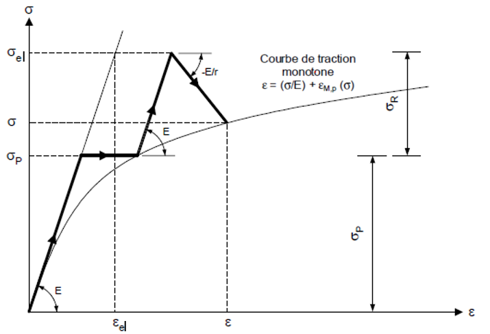
Image3.6-1: Reduction of the linear elastic stress \({\sigma }_{\mathit{el}}\) on the monotonic tensile curve
3.6.1. Abatement coefficients \(g\) and \({g}_{\mathit{opt}}\)#
A distinction is made between \(g\) and \({g}_{\mathit{opt}}\), calculated using the spring effect factor \({r}_{M}\) or its maximum according to the curvilinear abscissa \(\underset{s}{\mathit{max}}{r}_{M}\).
The coefficient \(g\) is calculated using the monotonic spring effect factor \({r}_{M}\), which depends on the curvilinear abscissa. The true stress and \(\sigma\) the true deformation \(ϵ\) are solutions of the following system of equations:
\({r}_{M}=-E\frac{ϵ-\frac{{\sigma }_{\mathit{ref}}+{\sigma }_{P}}{E}-{ϵ}_{M,p}({\sigma }_{P})}{\sigma -{\sigma }_{\mathit{ref}}-{\sigma }_{P}}\)
\(ϵ=\frac{\sigma }{E}+{ϵ}_{M,p}(\sigma )\)
where \({\sigma }_{P}\) corresponds to the stress induced by the internal pressure of the pipe, for example:
\({\sigma }_{P}=\mathrm{0,87}P\frac{{D}_{i}}{2{h}_{c}}\)
with \(P\), the internal pressure, \({D}_{i}\) the internal diameter, and \({h}_{c}\) the thickness of the pipe.
Inequality \({\sigma }_{P}<\sigma\) must be verified to ensure that \(g\) is calculated correctly.
The reduction coefficient is then written as:
\(g=\frac{\sigma -{\sigma }_{P}}{{\sigma }_{\mathit{ref}}}\),
The coefficient \({g}_{\mathit{opt}}\) is calculated in the same way as \(g\), but this time using the maximum monotonic spring effect factor \(\underset{s}{\mathit{max}}{r}_{M}\), no longer dependent on the curvilinear abscissa, but still dependent on the edge. The true stress \(\sigma\) and the true deformation \(ϵ\) are then solutions to the following system of equations:
\(\underset{s}{\mathit{max}}{r}_{M}=-E\frac{ϵ-\frac{{\sigma }_{\mathit{ref}}+{\sigma }_{P}}{E}-{ϵ}_{M,p}({\sigma }_{P})}{\sigma -{\sigma }_{\mathit{ref}}-{\sigma }_{P}}\)
\(ϵ=\frac{\sigma }{E}+{ϵ}_{M,p}(\sigma )\)
The reduction coefficient is then written as:
\({g}_{\mathit{opt}}=\frac{\sigma -{\sigma }_{P}}{{\sigma }_{\mathit{ref}}}\).
3.6.2. Abatement coefficients \({g}_{S}\) and \({g}_{\mathit{Sopt}}\)#
A distinction is made between \({g}_{S}\) and \({g}_{\mathit{Sopt}}\), calculated using the seismic spring effect factor \({r}_{S}\) or its maximum according to the curvilinear abscissa \(\underset{s}{\mathit{max}}{r}_{S}\).
The coefficient \({g}_{S}\) is calculated using the seismic spring effect factor \({r}_{S}\), depending on the curvilinear abscissa. True stress \(\sigma\) and true deformation \(ϵ\) are solutions of the following system of equations:
\({r}_{S}=-E\frac{ϵ-\frac{{\sigma }_{\mathit{ref}}+{\sigma }_{P}}{E}-{ϵ}_{M,p}({\sigma }_{P})}{\sigma -{\sigma }_{\mathit{ref}}-{\sigma }_{P}}\)
\(ϵ=\frac{\sigma }{E}+{ϵ}_{M,p}(\sigma )\)
The reduction coefficient is then written as:
\({g}_{S}=\frac{\sigma -{\sigma }_{P}}{{\sigma }_{\mathit{ref}}}\)
the coefficient \({g}_{\mathit{opt}}\) is calculated in the same way as \(g\), but this time using the maximum spring effect factor \(\underset{s}{\mathit{max}}{r}_{S}\), no longer depending on the curvilinear abscissa, but still depending on the section.
The true stress \(\sigma\) and the true deformation \(ϵ\) are then solutions to the following system of equations:
\(\underset{s}{\mathit{max}}{r}_{S}=-E\frac{ϵ-\frac{{\sigma }_{\mathit{ref}}+{\sigma }_{P}}{E}-{ϵ}_{M,p}({\sigma }_{P})}{\sigma -{\sigma }_{\mathit{ref}}-{\sigma }_{P}}\)
\(ϵ=\frac{\sigma }{E}+{ϵ}_{M,p}(\sigma )\)
The reduction coefficient is then written as:
\({g}_{\mathit{Sopt}}=\frac{\sigma -{\sigma }_{P}}{{\sigma }_{\mathit{ref}}}\).
3.7. Calculation of the reduction coefficients \({g}_{\mathit{RX}}\) and \({g}_{\mathit{SRX}}\), for each section (case RCCM_RX =” OUI “)#
In this case, it is considered that the true stress is no longer an unknown of the system of 2 equations, but a constant depending on an admissible stress defined from the data of the minimum breaking stress and the minimum stress at 0.2% of deformation of the material, the reduction coefficient can then be calculated directly without solving the system, by an analytical formula codified in the RCC -Mrx.
3.7.1. Calculating the true stress from an allowable stress#
The allowable constraint \({S}^{\text{*}}\) is defined by:
\({S}^{\text{∗}}=\alpha [\mathrm{0,426}{({R}_{p\mathrm{0,2}})}_{\mathit{min}}({\theta }_{m})+\mathrm{0,032}{({R}_{m})}_{\mathit{min}}({\theta }_{m})]\)
Where:
\(\alpha\) is a dimensionless coefficient greater than or equal to 1, it corresponds to the operand COEF of the material POST_ROCHE
\({({R}_{p\mathrm{0,2}})}_{\mathit{min}}({\theta }_{m})\) is the minimum conventional elastic limit at 0.2% deformation, for the average temperature \({\theta }_{m}\) in the thickness during the loading studied, it corresponds to the operand RP02_MIN of the material POST_ROCHE
\({({R}_{m})}_{\mathit{min}}({\theta }_{m})\) is the minimum tensile strength, for the average temperature \({\theta }_{m}\) in the thickness during the loading studied, it corresponds to the operand RM_MIN of the material POST_ROCHE
The true constraint \(\sigma\) is then defined by:
\(\sigma =2{S}^{\text{∗}}\raisebox{1ex}{{({R}_{p\mathrm{0,2}})}_{\mathit{moy}}({\theta }_{m})}\!\left/ \!\raisebox{-1ex}{{({R}_{p\mathrm{0,2}})}_{\mathit{min}}({\theta }_{m})}\right.\)
With:
\({({R}_{p\mathrm{0,2}})}_{\mathit{moy}}({\theta }_{m})\) the average conventional elastic limit at 0.2% deformation, for the average temperature \({\theta }_{m}\) in the thickness during the loading studied
Calculation of monotonic \({g}_{\mathit{RX}}\) and seismic \({g}_{\mathit{SRX}}\) abatement coefficients ~~~~~~~~~~~~~~~~~~~~~~~~~~~~~~~~~~~~~~~~~~~~~~~~~~~~~~~~~~~~~~~~~~~~~~~~~~~~~~~~~~~~~~~~~~~~~~~~~~~~~~~~~~~~~~~~~~~~~~~~~~~~~~~~~~~~~~~~~~~~~~~~~~~~~~~~~~~~~~~~~~~~~~~~~~~~~~~~~~~~~~~~~~~~~~~ ~~~~~~~~~~~~~~~
According to the codification RCC - MRx (RB 3651.1132 and RB 3651.1142) the monotonic and seismic reduction coefficients are then as follows:
\({g}_{\mathit{RX}}=\frac{(\sigma -{\sigma }_{P})(1+\underset{s}{\mathit{max}}{r}_{M})}{E[{\epsilon }_{M,p}(\sigma )-{\epsilon }_{M,p}({\sigma }_{P})]+(\sigma -{\sigma }_{P})(1+\underset{s}{\mathit{max}}{r}_{M})}\)
and
\({g}_{\mathit{SRX}}=\frac{(\sigma -{\sigma }_{P})(1+\underset{s}{\mathit{max}}{r}_{S})}{E[{\epsilon }_{M,p}(\sigma )-{\epsilon }_{M,p}({\sigma }_{P})]+(\sigma -{\sigma }_{P})(1+\underset{s}{\mathit{max}}{r}_{S})}\)
In the following, the treatment is the same regardless of the value of RCCM_RX. So \({g}_{\mathit{RX}}\) will correspond to \({g}_{\mathit{opt}}\) and \({g}_{\mathit{SRX}}\) to \({g}_{\mathit{Sopt}}\).
3.8. Calculation of equivalent stresses#
3.8.1. General case#
The equivalent stress is obtained by combining the moments obtained in § 3.2.1 weighted by the reduction coefficients.
The coefficients \(g\) and \({g}_{S}\) are then used to obtain the equivalent constraint (this value is not calculated in the case RCCM_RX =” OUI “):
- math:
{sigma} _ {mathit {eq}} =sqrt {{left ({D} _ {1}frac {P {D} _ {i}} {2 {h} _ {C}}right)} {C}}}right)}}right)}} ^ {2}}right)} ^ {2}}right)} ^ {2}}right)} ^ {2}}right)} ^ {2}}right)} ^ {2}}right)} ^ {2}}right)} ^ {2}}right)} ^ {2}}right)} ^ {2}}right)} ^ {2}}right)} ^ {2}}right)} ^ {2}}right left|mright|+ {g} _ {S}left| {m} _ {mathit {SI}}right|⟩}} ^ {2}}},
or the coefficients \({g}_{\mathit{opt}}\) and \({g}_{\mathit{Sopt}}\) to obtain the optimized equivalent stress:
- math:
{{sigma} _ {mathit {eq}}}}} _ {mathit {opt}} =sqrt {{left ({D} _ {1}frac {P {D} _ {D} _ {i} _ {i}}}} {i}}}} {i}}} {i}}} {i}}} {i}}} {2}}} {2}right)} ^ {2}} +frac {1} {Z} {2}, {(left|mright|+ {g} | + {g} _ {mathit {opt}}}left|mright|+ {g} _ {mathit {Sopt}}}left| {m} | {m}} _ {m} _ {m} _ {m} _ {m} _ {m} _ {m} _ {m} _ {m} _ {m} _ {m} _ {mathit {SI}}}right|)} ^ {2} ⟩}},
where:
- math:
left|Mright|=left (begin {array} {c} {M} _ {1}\ {M} _ {2}\ {M} _ {3}end {array}right|= =end {array}right) = =left (left (left) (left) (left) (begin {array}\{array}right) = =left (left) (begin {array}right) =left (begin {array}right) =left (begin {array}right) is the sum of the moments dependent on the efforts, including the contribution of the primary loads (weight…) _ {2}\ {M} _ {3}end {array}\{right}), taken in absolute values,
- math:
left|mright|=left (begin {array} {c} {m} _ {1}\ {m} _ {2}\ {m} _ {3}end {array}right|= =left (end {array}right) is the sum of the moments dependent on the movements (thermal expansion, seismic differential movements), taken in absolute values,
- math:
left| {m} _ {mathit {SI}}right|=left (begin {array} {c} {{m} _ {mathit {SI}}}}}} _ {1}\ {{m}} _ {1}{{m}} _ {1}{{m}}} _ {1}{{m}}} _ {3} _ {1}{{m}}} _ {3}end {array}right) is the moment corresponding to the dynamic part of the inertial earthquake, classified as dependent on movements, taken in absolute value,
\(P\) is the pressure imposed inside the pipe,
\({D}_{i}\) and \({h}_{c}\) correspond respectively to the inner diameter and to the thickness of the pipe,
\(Z\) is the moment of inertia (which is written for \(Z=\frac{{I}_{y}}{R}\) circular beams),
\({D}_{1}\) is the stress coefficient associated with internal pressure,
\({D}_{2}=\left(\begin{array}{c}{D}_{21}\\ {D}_{22}\\ {D}_{23}\end{array}\right)\) are the stress coefficients associated with torsional moments (\({D}_{21}\)) and flexural moments (\({D}_{22}\) and \({D}_{23}\)),
\(⟨\mathrm{.},\mathrm{.}⟩\) is the dot product.
3.8.2. Case of straight pipes#
In the case of straight pipes, we install:
\({D}_{1}=0\),
\({D}_{21}=0.712\),
\({D}_{22}={D}_{23}=0.429{(\frac{{D}_{e}}{{h}_{c}})}^{0.16}\),
where \({D}_{e}\) is the outside diameter of the pipe.
3.8.3. Case of discounts#
In the case of discounts, we ask:
\(Z=\mathit{min}\frac{{I}_{y}}{R}\)
\({D}_{1}=0\),
\({D}_{21}=0.712\),
\({D}_{22}={D}_{23}=0.429{(\mathit{max}\frac{{D}_{e}}{{h}_{c}})}^{0.16}\),
where \(\mathit{min}\frac{{I}_{y}}{R}\) is the minimum of the ratio and \(\mathit{max}\frac{{D}_{e}}{{h}_{c}}\) is the maximum of the ratio on the pipe element.
3.8.4. Case of bent pipes and bends#
In the case of elbows, we apply:
\({D}_{1}=0.87\),
\({D}_{21}=0.712\),
\({D}_{22}=\mathit{max}(1.07{(\frac{\pi }{{\psi }_{c}})}^{-0.4}{f}^{-2/3}{(1+0.142\frac{{\mathit{PD}}_{i}}{2{h}_{c}{S}_{y}{f}^{1.45}})}^{-1},1.02)\),
\({D}_{23}=\mathit{max}(0.809{f}^{-0.44}{(1+0.142\frac{{\mathit{PD}}_{i}}{2{h}_{c}{S}_{y}{f}^{1.45}})}^{-1},1.02)\),
\(f={h}_{c}\frac{{R}_{c}}{{r}_{m}^{2}}\) where \({r}_{m}=\frac{{D}_{e}-{h}_{c}}{2}\),
\({D}_{i}\), \({D}_{e}\), and \({h}_{c}\) correspond to the inner, outer and outer diameters, and pipe thickness respectively.
\({S}_{y}\) is the conventional minimum elastic limit at 0.2% deformation (Pa) (given by the user)
\({R}_{c}\) is the radius of curvature (given by the user),
\({\psi }_{c}\) is the opening angle of the elbow (given by the user).