2. Numerical aspects of limit load calculation#
2.1. Norton-Hoff behavior relationship#
The stress tensor \(\sigma (u)\) verifies the Norton-Hoff behavior relationship. The stress deflector associated with the deformation rate is:
\({\mathrm{\sigma }}^{D}\left(\mathrm{u}\right)=A\left(m\right)\text{.}{\left(\sqrt{{\mathrm{\epsilon }}^{D}\left(\mathrm{u}\right)\text{.}{\mathrm{\epsilon }}^{D}\left(\mathrm{u}\right)}\right)}^{m\text{-}2}\text{.}{\mathrm{\epsilon }}^{D}\left(\mathrm{u}\right)\) eq 2.1-1
with \(\text{tr}\varepsilon (u)=0\), and: \(A(m)={k}^{1\text{-}m}{(\frac{2}{3})}^{m/2}{\sigma }_{y}^{m}\).
This behavior is integrated in the same way as the incremental elastoplastic behaviors of Von Mises [R5.03.02]. Note, however, that, at an integration point, the calculation of the stress tensor as a function of the strain tensor is explicit, no iterative schema being used. In addition, no internal variables are required to integrate this behavior.
In Code_Aster, the calculation of the limit load being independent of the elasticity coefficients , we choose \(k={\sigma }_{y}\), from where \(A(m)={\sigma }_{y}{(\frac{2}{3})}^{m/2}\). We thus find the incompressible elastic problem when \(m=2\), for a Young’s modulus \(E={\sigma }_{y}\).
In addition, the sequence of scalars \(m\) is directly deduced from the list of (fictional) calculation times by:
\(m=1+{\text{10}}^{1\text{-}t}\),
so that when the moment increases, \(m\) tends to 1, and the behavior approaches perfect rigid-plastic behavior, see in one-dimensional curves [fig. 2.1-a]. In practice, we choose the sequence of values in [tab. 2.1-a].
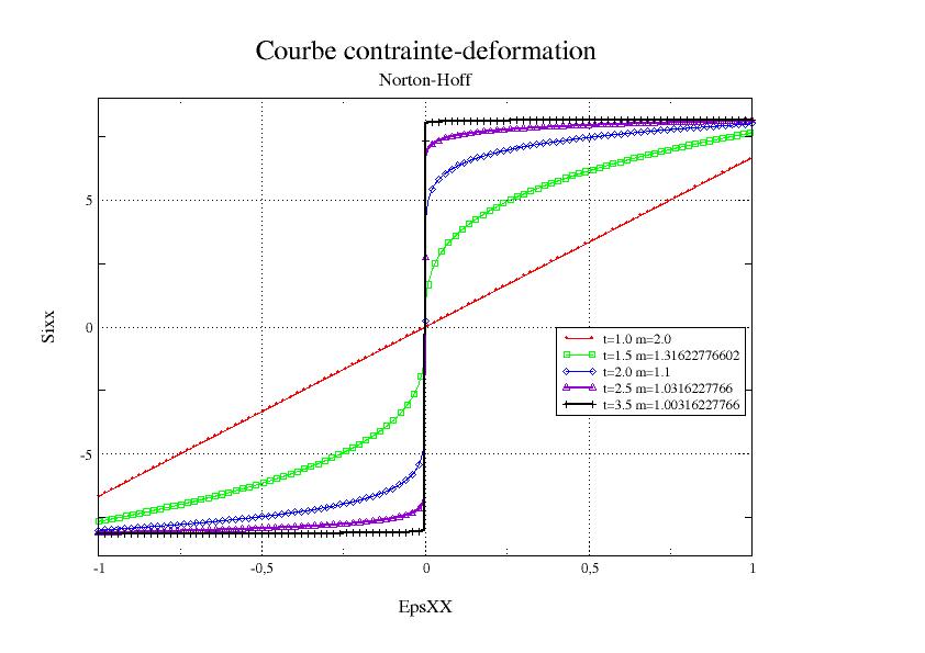
Fig. 2.1-a. Stress-strain curve for various values from time \(t\).
1 |
1.5 |
1.7 |
2 |
… |
||
2 |
1.3 |
1.2 |
1.1 |
… |
1 |
|
Tab. 2.1-a. Continued values from time \(t\), and corresponding \(m\) values.
The tangent operator, used in option FULL_MECA of Newton’s method, is written using [éq 2.1-1]:
\({\begin{array}{c}\frac{d{\sigma }^{D}}{d{\varepsilon }^{D}}\end{array}\mid }_{\varepsilon (u)}=A(m){\parallel {\varepsilon }^{D}\parallel }^{m\text{-}2}(\text{Id}\otimes \text{Id}+(m-2){\parallel {\varepsilon }^{D}\parallel }^{-2}{\varepsilon }^{D}\otimes {\varepsilon }^{D})\) eq 2.1-2
with \({\varepsilon }^{D}\), \({\sigma }^{D}\) the vectors of deviatory deformations and constraints written in vector notations of WALPOLE - COWIN:
\({\varepsilon }^{D}=({\varepsilon }_{11}^{D},{\varepsilon }_{22}^{D},{\varepsilon }_{33}^{D},\sqrt{2}{\varepsilon }_{12}^{D},\sqrt{2}{\varepsilon }_{23}^{D},\sqrt{2}{\varepsilon }_{31}^{D})\)
\({\sigma }^{D}=({\sigma }_{11}^{D},{\sigma }_{22}^{D},{\sigma }_{33}^{D},\sqrt{2}{\sigma }_{12}^{D},\sqrt{2}{\sigma }_{23}^{D},\sqrt{2}{\sigma }_{31}^{D})\)
2.2. Piloting#
The problem is written in variational form as follows on the space of incompressible fields.
For \(m\) given, so at a given time \(t\), knowing the solution at the previous moment (noted \({u}^{-},{\lambda }^{-}\)), find \((\Delta \lambda ,\Delta u)\in \mathrm{IR}\times \tilde{{V}_{a}}\) such as:
\(\{\begin{array}{}{\int }_{\Omega }\sigma ({u}^{-}+\Delta u)\text{.}\varepsilon (v)d\Omega ={L}_{0}(v)+({\lambda }^{-}+\Delta \lambda )L(v)\forall v\in {\tilde{}V}_{0}\\ L(v)={\int }_{\Omega }f\text{.}vd\Omega +{\int }_{{\Gamma }_{f}}F\text{.}v\text{dS}=1\end{array}\) eq 2.2-1
\({L}_{0}\) is the permanent load and \(L\) the load controlled by the parameter \(\lambda\), cf. [§1.1],
\(\tilde{{V}_{0}}\) is a space of discretized functions based on incompressible finite elements, and is therefore defined by a \((U)\) vector of degrees of freedom.
This problem allows for a single solution for all \(1\le m\le 2\) (see [bib4]). For \(m=2\) the problem is of the incompressible linear elasticity type.
The discretized problem at moment \(t\) (so for a value of \(m\), cf. [tab. 2.1-a]) can be written (omitting the boundary conditions to simplify):
\(\{\begin{array}{}{F}_{\text{int}}(\Delta U;{U}^{-};\text{.}\text{.})={F}_{0}^{\text{ext}}+\lambda {F}^{\text{ext}}\\ L({U}^{-}+\Delta U)=1\end{array}\)
The search for \(\lambda\) ensuring the condition \(L(U)=1\) is ensured by a control algorithm [R5.03.80].
Briefly, the principle is as follows: by linearizing the equations relating to internal forces, we obtain, for iteration \(n\) of Newton’s algorithm, cf. [R5.03.01]:
\(\underset{{K}_{T}}{\underset{\underbrace{}}{\left[\frac{\partial {F}_{\text{int}}}{\partial U}(\Delta {U}^{n})\right]}}\left[\delta U\right]=\underset{{R}^{\text{cst}}}{\underset{\underbrace{}}{\left[{F}_{0}^{\text{ext}}-{F}_{\text{int}}(\Delta {U}^{n})\right]}}+\lambda \underset{{R}^{\text{pilo}}}{\underset{\underbrace{}}{\left[{F}^{\text{ext}}\right]}}\) eq 2.2-2
We can now express the corrections of movements \(\delta U\) and Lagrange multipliers \(\delta \lambda\) as a function of \(\lambda\) by resolving this linear system:
\(\left[\delta U\right]=\left[\delta {U}^{\text{cst}}\right]+\lambda \left[\delta {U}^{\text{pilo}}\right]\text{où}\left[\delta {U}^{\text{cst}}\right]={K}_{{T}^{-1}}{R}^{\text{cst}}\text{et}\left[\delta {U}^{\text{pilo}}\right]={K}_{{T}^{-1}}{R}^{\text{pilo}}\) eq 2.2-3
We can substitute the displacement correction \(\delta U\) according to its expression [éq2.2-2] in the control equation for controlling the control of the system \(L(U)=1\); the result is a scalar equation in \(\Delta \lambda\):
\(L({U}^{-}+\Delta {U}^{n}+\delta {U}^{\text{cst}}+\lambda \delta {U}^{\text{pilo}})=1\) be
\({\int }_{\Omega }f\text{.}({U}^{-}+\Delta {U}^{n}+\delta {U}^{\text{cst}}+\lambda \delta {U}^{\text{pilo}})d\Omega +{\int }_{{\Gamma }_{f}}F\text{.}({U}^{-}+\Delta {U}^{n}+\delta {U}^{\text{cst}}+\lambda \delta {U}^{\text{pilo}})\text{dS}=1\) eq 2.2-4
which in discretized form amounts to:
\(\begin{array}{}\\ \sum _{e}{F}^{\text{ext}}\text{.}({U}^{-}+\Delta {U}^{n}+\delta {U}^{\text{cst}}+\lambda \delta {U}^{\text{pilo}})=1\end{array}\)
which leads to:
\(\lambda =\frac{1-\sum _{e}{F}^{\text{ext}}\text{.}({U}^{-}+\Delta {U}^{n}+\delta {U}^{\text{cst}})}{\sum _{e}{F}^{\text{ext}}\text{.}\delta {U}^{\text{pilo}}}\) eq 2.2-5
2.3. Post-processing of the limit load calculation#
Having obtained solution \(({\lambda }_{m},{u}_{m})\), for each moment, therefore each given \(m\), it remains to use the series of \({\lambda }_{m}\) to build the approximation of the limit load. To do this, we exploit the properties [éq 1.3-2], [éq 1.3-3], the fact that \(A(m)\) is increasing and the property resulting from minimization [éq 1.3-2] (see [bib7]).
From these last two, with \(1\le r\le s\), we deduce that for \({u}_{r}\) and \({u}_{s}\) respective solutions (also verifying the condition of incompressibility and normalization) of [éq 1.3-2] for \(m=r\) and
:
\(({\int }_{\Omega }A(r){(\varepsilon ({u}_{r})\text{.}\varepsilon ({u}_{r}))}^{r/2}d\Omega )\le ({\int }_{\Omega }A(s){(\varepsilon ({u}_{s})\text{.}\varepsilon ({u}_{s}))}^{s/2}d\Omega )\)
Associated with the [éq 1.3-3] property, we shoot for \(1\le r\le s\), noting \({\parallel \Omega \parallel }_{r}={\int }_{\Omega }A(r)d\Omega\):
\({\int }_{\Omega }A(r)\sqrt{\varepsilon ({u}_{r})\text{.}\varepsilon ({u}_{r})}d\Omega \le {\parallel \Omega \parallel }_{r}^{1\text{-}\frac{1}{r}}{({\int }_{\Omega }A(r){(\varepsilon ({u}_{r})\text{.}\varepsilon ({u}_{r}))}^{r/2}d\Omega )}^{\frac{1}{r}}\le {\parallel \Omega \parallel }_{s}^{1\text{-}\frac{1}{s}}{({\int }_{\Omega }A(s){(\varepsilon ({u}_{s})\text{.}\varepsilon ({u}_{s}))}^{s/2}d\Omega )}^{\frac{1}{s}}\) eq 2.3-1
In fact, this property results from the inclusion of functional spaces \({L}^{r}\supset {L}^{s}\), for \(1\le r\le s\), or also, where \(h(x)\) plays the role of a variable measure (conditioned by the resistance limit \({\sigma }_{y}\)):
\({\parallel \Omega \parallel }_{r}^{-\frac{1}{r}}{({\int }_{\Omega }h(x){\mid f(x)\mid }^{r}d\Omega )}^{\frac{1}{r}}\le {\parallel \Omega \parallel }_{s}^{-\frac{1}{s}}{({\int }_{\Omega }h(x){\mid f(x)\mid }^{s}d\Omega )}^{\frac{1}{s}}\)
We note the terms \({\tilde{\lambda }}_{m}\) of the following below, which are calculated in practice by post-treatment using \({u}_{m}\) (the external power being unitary):
\({\tilde{\lambda }}_{m}={\parallel \Omega \parallel }_{m}^{1-\frac{1}{m}}{({\int }_{\Omega }A(m){(\varepsilon ({u}_{m})\text{.}\varepsilon ({u}_{m}))}^{m/2}d\Omega )}^{\frac{1}{m}}\text{}-{L}_{0}({u}_{m})\) eq 2.3-2
This sequence \({\tilde{\lambda }}_{m}\) is therefore decreasing for \(m\to {1}^{+}\) and we show [bib7] that it converges to, which \({\lambda }_{\text{lim}}\) allows good control. How can we minimize (knowing that
) the first term of [éq 2.3-1]:
\({\lambda }_{\text{lim}}\le {\int }_{\Omega }{\sigma }_{y}\sqrt{\frac{2}{3}\varepsilon ({u}_{m})\text{.}\varepsilon ({u}_{m})}d\Omega \text{}-{L}_{0}({u}_{m})\le {\tilde{\lambda }}_{m}\)
So we calculate for each value of
(so from the moment \(t\)) the load limit \({\tilde{\lambda }}_{m}\) by excess also converging to \({\lambda }_{\text{lim}}\):
\({\lambda }_{\text{lim}}\le {\stackrel{ˆ}{\lambda }}_{m}={\int }_{\Omega }{\sigma }_{y}\sqrt{\frac{2}{3}\varepsilon ({u}_{m})\text{.}\varepsilon ({u}_{m})}d\Omega \text{}-{L}_{0}({u}_{m})\) eq 2.3-3
The quality of the approximation of the limit load \({\lambda }_{\text{lim}}\) is judged by comparing the various values of \({\tilde{\lambda }}_{m}\) which converge to \({\lambda }_{\text{lim}}\) by excess (in \(m\to {1}^{+}\)). These terms are calculated by numerical integration at the Gauss points of the finite elements.
Another interpretation of the interest that this series brings lies in the fact that it directly uses the expression of the support function of the resistance convex, that is to say the dispersible power in potential ruin modes, applied to incompressible and standardized solutions calculated \({u}_{m}\).
In the case where the permanent load is zero: \({L}_{0}\mathrm{=}0\), it is easy to exploit the stress field (almost statically admissible) calculated with the solution \({u}_{m}\) and obtain a value by estimating the limit load, which would necessarily be a true lower bound if the balance were verified exactly (see [bib4]).
We therefore calculate the sequence \({\underline{\lambda }}_{m}\), which, on the other hand, has no monotony properties:
\({\underline{\lambda }}_{m}={\int }_{\Omega }\frac{A(m)}{m}\text{.}{(\sqrt{\varepsilon ({u}_{m})\text{.}\varepsilon ({u}_{m})})}^{m}d\Omega \text{.}{(\underset{x\in \Omega }{\text{Sup}}(\frac{\sqrt{\frac{3}{2}{\sigma }^{D}({u}_{m})\text{.}{\sigma }^{D}({u}_{m})}}{{\sigma }_{y}}))}^{\text{-}1}\le {\stackrel{ˆ}{\lambda }}_{m}\) eq 2.3-4
This maximization (of the function called resistance convex gauge) is only calculated at the Gauss points of the finite elements. Also the value obtained, for each
, less than \({\tilde{\lambda }}_{m}\) [bib4], can only be considered as an indication.
On the other hand, always in the case where the permanent loads are zero, it makes it possible, with the excess value \({\tilde{\lambda }}_{m}\), to provide a framework for the limit load of the discretized problem.